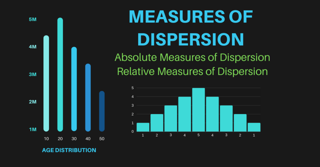
Measures of dispersion is second important topic after Measures of Central Tendency in Statistics. In this article, we are going to discuss Measures of Dispersion, Absolute Measures of Dispersion, Relative Measures of Dispersion, theoretically and numerically with the help of formulas and solved example questions for better understanding for both ungrouped and grouped data.
Table of Contents
Understanding Measures of Dispersion in Data Analysis
Introduction
Measures of dispersion calculate the spread, dispersion, or scatteredness of the data within the dataset around the average or central tendency. In other words, we can say that it calculates the variability. It presents a quantitative analysis that how values are spread around the central position of the data. In financial analysis, it is a very important measure that tells the investor about the risk associated with the investment. As the spread or variability is greater, the risk associated with that investment is also greater, and similarly, expected profit may also be greater or vice versa. Statisticians or data analysts not just rely on averages but also use variability analysis to confirm their predictions.
There are two types of dispersion one is called Absolute measures of dispersion and the other one is called relative measures of dispersion.
Absolute Measures of Dispersion
An Absolute measure of dispersion calculates the dispersion in terms of quantity while using units of the data and we can say that it calculates the variability in unit terms while ignoring central tendency.
Important Measures of Absolute Dispersion
Range
Range is an absolute measure of dispersion that is the difference between the highest and lowest values of the data.
Formula for ungrouped data
![\[ \mathbf{Xm - Xo}\ \]](https://bcfeducation.com/wp-content/ql-cache/quicklatex.com-57c488207abf7cb34f4c4d696830a4cc_l3.png "Rendered by QuickLaTeX.com")
Formula for grouped data
Quartile Deviation or Semi Interquartile Range
Quartile Deviation or Semi Interquartile Range focuses on the center of the data or 50% of the data. It is the fraction of the difference of Quartile 3 and Quartile 1 by 2. It is normally used in skewed data.
Formula for ungrouped data
![\[ \frac{\mathbf{Q}\mathbf{3 - Q}\mathbf{1}}{\mathbf{2}}\ \]](https://bcfeducation.com/wp-content/ql-cache/quicklatex.com-4f29a8af97e491179081452fd5b3a1c9_l3.png "Rendered by QuickLaTeX.com")
Formula for grouped data
![\[ \frac{\mathbf{Q}\mathbf{3 - Q}\mathbf{1}}{\mathbf{2}}\ \]](https://bcfeducation.com/wp-content/ql-cache/quicklatex.com-4b27536d758bf941ced529ea3495b426_l3.png "Rendered by QuickLaTeX.com")
Mean Deviation about Mean
Mean deviation through mean calculates the deviation of each X value of the data set around the mean while ignoring minus sign and it is an absolute measure of dispersion.
Formula for ungrouped data
![\[ \frac{\mathbf{\sum}\left| \mathbf{X -}\overline{\mathbf{X}} \right|}{\mathbf{n}}\ \]](https://bcfeducation.com/wp-content/ql-cache/quicklatex.com-692a877e3eb4949904a8ec7b9594c86f_l3.png "Rendered by QuickLaTeX.com")
Formula for grouped data
![\[ \frac{\mathbf{\sum f}\left| \mathbf{X -}\overline{\mathbf{X}} \right|}{\mathbf{\sum f}}\ \]](https://bcfeducation.com/wp-content/ql-cache/quicklatex.com-119b9cc724851c1ed2acde6d9e11e2ef_l3.png "Rendered by QuickLaTeX.com")
Mean Deviation about Median
Mean deviation through median calculates the deviation of each X value of the data set around the median while ignoring minus sign and it is an absolute measure of dispersion.
Formula for ungrouped data
![\[ \frac{\mathbf{\sum}\left| \mathbf{X -}\widetilde{\mathbf{X}} \right|}{\mathbf{n}}\ \]](https://bcfeducation.com/wp-content/ql-cache/quicklatex.com-d3e277620d2d608766adde169266cf62_l3.png "Rendered by QuickLaTeX.com")
Formula for grouped data
![\[ \frac{\mathbf{\sum f}\left| \mathbf{X -}\widetilde{\mathbf{X}} \right|}{\mathbf{\sum f}}\ \]](https://bcfeducation.com/wp-content/ql-cache/quicklatex.com-17e83bfb53590f183e1f4e0b49dcff8c_l3.png "Rendered by QuickLaTeX.com")
Mean Deviation about Mode
Mean deviation through median calculates the deviation of each X value of the data set around the mode while ignoring minus sign and it is an absolute measure of dispersion.
Formula for ungrouped data
![\[ \frac{\mathbf{\sum}\left| \mathbf{X -}\widehat{\mathbf{X}} \right|}{\mathbf{n}}\ \]](https://bcfeducation.com/wp-content/ql-cache/quicklatex.com-fc520b3c11640af7119410a452d42e78_l3.png "Rendered by QuickLaTeX.com")
Formula for grouped data
![\[ \frac{\mathbf{\sum f}\left| \mathbf{X -}\widehat{\mathbf{X}} \right|}{\mathbf{\sum f}}\ \]](https://bcfeducation.com/wp-content/ql-cache/quicklatex.com-542d52851c6aa8257fb46bb14845d5e8_l3.png "Rendered by QuickLaTeX.com")
Standard Deviation
Standard Deviation is very important measure of dispersion and it is widely used measure of dispersion. It is square root of average squared deviation from the arithmetic mean of the dataset. It calculates the variability present in the dataset.
Formula for ungrouped data
![\[ \sqrt{\left( \frac{\mathbf{\sum}\mathbf{X}^{\mathbf{2}}}{\mathbf{n}} \right)\mathbf{-}\left( \frac{\mathbf{\sum X}}{\mathbf{n}} \right)^{\mathbf{2}}}\ \]](https://bcfeducation.com/wp-content/ql-cache/quicklatex.com-9eb43a831d081421f3cb23b9edd21e8d_l3.png "Rendered by QuickLaTeX.com")
Formula for grouped data
![\[ \sqrt{\left( \frac{\mathbf{\sum f}\mathbf{x}^{\mathbf{2}}}{\mathbf{\sum f}} \right)\mathbf{-}\left( \frac{\mathbf{\sum fx}}{\mathbf{\sum f}} \right)^{\mathbf{2}}}\ \]](https://bcfeducation.com/wp-content/ql-cache/quicklatex.com-43c0449dd59f84a818cc05d5f7e045ba_l3.png "Rendered by QuickLaTeX.com")
Variance
Variance is also very important measure of dispersion and it is widely used measure of dispersion. It is simply the average squared deviation from the arithmetic mean of the dataset. It calculates the variability present in the dataset.
Formula for ungrouped data
![\[ \left( \frac{\mathbf{\sum}\mathbf{X}^{\mathbf{2}}}{\mathbf{n}} \right)\mathbf{-}\left( \frac{\mathbf{\sum X}}{\mathbf{n}} \right)^{\mathbf{2}}\ \]](https://bcfeducation.com/wp-content/ql-cache/quicklatex.com-45753aedbb7d6703e204e9734d1bc6cc_l3.png "Rendered by QuickLaTeX.com")
Formula for grouped data
![\[ \left( \frac{\mathbf{\sum f}\mathbf{x}^{\mathbf{2}}}{\mathbf{\sum f}} \right)\mathbf{-}\left( \frac{\mathbf{\sum fx}}{\mathbf{\sum f}} \right)^{\mathbf{2}}\ \]](https://bcfeducation.com/wp-content/ql-cache/quicklatex.com-ad43c80d147f37b6ac53f54fa3136f7b_l3.png "Rendered by QuickLaTeX.com")
Relative Measures of Dispersion
Relative measures of dispersion calculates the dispersion of the dataset with respect to central tendency. It is a percentage based measure of dispersion. Simply, we can say that it calculates the dispersion in relative terms. There are different relative measures of dispersion discussed below:
Important Measures of Absolute Dispersion
Coefficient of Range
Coefficient of Range is a relative measure of dispersion that is the quotient of the negative and positive difference between the highest and lowest values of the data.
Formula for ungrouped data
![\[ \frac{\mathbf{Xm - Xo}}{\mathbf{Xm + Xo}}\ \]](https://bcfeducation.com/wp-content/ql-cache/quicklatex.com-0ed70b09fbfa43e3a57169a088dae411_l3.png "Rendered by QuickLaTeX.com")
Formula for grouped data
![\[ \frac{\mathbf{Xm - Xo}}{\mathbf{Xm + Xo}}\ \]](https://bcfeducation.com/wp-content/ql-cache/quicklatex.com-785faa6bab8fb721b345f5f647ae19cb_l3.png "Rendered by QuickLaTeX.com")
Coefficient of Quartile Deviation
Coefficient of Quartile Deviation is a relative measure of dispersion that focuses on the center of the dataset. It is the negative and positive fraction of the difference of Quartile 3 and Quartile 1. It is normally used in skewed data.
Formula for ungrouped data
![\[ \frac{\mathbf{Q}\mathbf{3 - Q}\mathbf{1}}{\mathbf{Q}\mathbf{3 + Q}\mathbf{1}}\ \]](https://bcfeducation.com/wp-content/ql-cache/quicklatex.com-93956723688326ce7771a1eceb084d1e_l3.png "Rendered by QuickLaTeX.com")
Formula for grouped data
Coefficient of Mean Deviation through Mean
The coefficient of Mean deviation through the mean is a relative measure of dispersion that calculates the deviation of each X value of the data set around the mean while ignoring the minus sign in relative terms. It is the quotient of Mean deviation through mean and mean.
Formula for ungrouped data
![\[ \frac{\mathbf{Mean\ Deviation\ through\ Mean}}{\mathbf{Mean}}\ \]](https://bcfeducation.com/wp-content/ql-cache/quicklatex.com-baf2dac31e621e5b21c82901cbce472b_l3.png "Rendered by QuickLaTeX.com")
Formula for grouped data
Coefficient of Mean Deviation through Median
The coefficient of Mean deviation through the median is a relative measure of dispersion that calculates the deviation of each X value of the data set around the median while ignoring the minus sign in relative terms. It is the quotient of Mean deviation through median and median.
Formula for ungrouped data
![\[ \frac{\mathbf{Mean\ Deviation\ through\ Median}}{\mathbf{Median}}\ \]](https://bcfeducation.com/wp-content/ql-cache/quicklatex.com-7bc5fc61f4bbd6127404b6f495b51f16_l3.png "Rendered by QuickLaTeX.com")
Formula for grouped data
Coefficient of Mean Deviation through Mode
The coefficient of Mean deviation through the mode is a relative measure of dispersion that calculates the deviation of each X value of the data set around the mode while ignoring the minus sign in relative terms. It is the quotient of Mean deviation through mode and mode.
Formula for ungrouped data
![\[ \frac{\mathbf{Mean\ Deviation\ through\ Mode}}{\mathbf{Mode}}\ \]](https://bcfeducation.com/wp-content/ql-cache/quicklatex.com-58b440efa8648b96a67e6e649521a150_l3.png "Rendered by QuickLaTeX.com")
Formula for grouped data
![\[ \frac{\mathbf{Mean\ Deviation\ through\ Mode}}{\mathbf{Mode}}\ \]](https://bcfeducation.com/wp-content/ql-cache/quicklatex.com-89c8498910c6750d04f4823dd62f6ee6_l3.png "Rendered by QuickLaTeX.com")
Coefficient of Standard Deviation
As we discussed above, Standard Deviation is a very important measure of dispersion and it is a widely used measure of dispersion. It is the square root of the average squared deviation from the arithmetic mean of the dataset. It calculates the variability present in the dataset. On the other hand coefficient of standard deviation tells us the same variability in relative terms.
Formula for ungrouped data
![\[ \frac{\mathbf{Standard\ Deviation}}{\mathbf{Mean}}\ \]](https://bcfeducation.com/wp-content/ql-cache/quicklatex.com-57be0631b3d5bd6227dc419c03e36c0b_l3.png "Rendered by QuickLaTeX.com")
Formula for grouped data
Coefficient of Variation
As we discussed above, the variance is also a very important measure of dispersion and it is widely used measure of dispersion. It is simply the average squared deviation from the arithmetic mean of the dataset. It calculates the variability present in the dataset. On the other hand coefficient of variation tells us the variability calculated by variance in relative terms.
Formula for ungrouped data
![\[ \frac{\mathbf{Standard\ Deviation}}{\mathbf{Mean}}\mathbf{\times 100}\ \]](https://bcfeducation.com/wp-content/ql-cache/quicklatex.com-f6b92eed8662b34a94361879efbf4824_l3.png "Rendered by QuickLaTeX.com")
Formula for grouped data

Practical Example Questions for Understanding
Example Solved Question for Ungrouped Data
We have a data containing marks of the 10 students in the subject of Statistics given below:
| Students | 1 | 2 | 3 | 4 | 5 | 6 | 7 | 8 | 9 | 10 |
| Marks | 50 | 70 | 65 | 80 | 45 | 90 | 80 | 40 | 30 | 25 |
Calculate all measures of dispersion both absolute and relative measures.
Solution:
First step is to arrange the data into ascending form:
| S/No | Marks (X) | | | | |
| 1 | 25 | 32.5 | 36.25 | 55 | 625 |
| 2 | 30 | 27.5 | 31.25 | 50 | 900 |
| 3 | 40 | 17.5 | 21.25 | 40 | 1600 |
| 4 | 45 | 12.5 | 16.25 | 35 | 2025 |
| 5 | 50 | 7.5 | 11.25 | 30 | 2500 |
| 6 | 65 | 7.5 | 3.75 | 15 | 4225 |
| 7 | 70 | 12.5 | 8.75 | 10 | 4900 |
| 8 | 80 | 22.5 | 18.75 | 0 | 6400 |
| 9 | 80 | 22.5 | 18.75 | 0 | 6400 |
| 10 | 90 | 32.5 | 28.75 | 10 | 8100 |
| ∑X=575 | | | | |
![\[ \left| \mathbf{X -}\overline{\mathbf{X}} \right|\ \]](https://bcfeducation.com/wp-content/ql-cache/quicklatex.com-6c20ffb663a8347e69f2fca9db808884_l3.png "Rendered by QuickLaTeX.com")
![\[ \left| \mathbf{X -}\widetilde{\mathbf{X}} \right|\ \]](https://bcfeducation.com/wp-content/ql-cache/quicklatex.com-ec5fe55a9ab72f079158aeabd02276c7_l3.png "Rendered by QuickLaTeX.com")
![\[ \left| \mathbf{X -}\widehat{\mathbf{X}} \right|\ \]](https://bcfeducation.com/wp-content/ql-cache/quicklatex.com-08c180237fb1716433b37d6efe0164d0_l3.png "Rendered by QuickLaTeX.com")
![\[ \mathbf{X}^{\mathbf{2}}\ \]](https://bcfeducation.com/wp-content/ql-cache/quicklatex.com-f9ddc9ffd4e92f48270c6fddc7b8c553_l3.png "Rendered by QuickLaTeX.com")
![\[ \mathbf{\sum}\left| \mathbf{X -}\overline{\mathbf{X}} \right|\textbf{=195} \]](https://bcfeducation.com/wp-content/ql-cache/quicklatex.com-963e0b54ac60ab20701205c47ae3f41a_l3.png "Rendered by QuickLaTeX.com")
![\[ \mathbf{\sum}\left| \mathbf{X -}\widetilde{\mathbf{X}} \right|\mathbf{=}\textbf{195} \]](https://bcfeducation.com/wp-content/ql-cache/quicklatex.com-645522b819e8fb41509b7e1d57be713b_l3.png "Rendered by QuickLaTeX.com")
![\[ \mathbf{\sum}\left| \mathbf{X -}\widehat{\mathbf{X}} \right|\mathbf{=}\textbf{245} \]](https://bcfeducation.com/wp-content/ql-cache/quicklatex.com-0cd1cd214591f25b50b2ca778353f421_l3.png "Rendered by QuickLaTeX.com")
![\[ \mathbf{\sum}\mathbf{X}^{\mathbf{2}}\mathbf{= \ }\textbf{37675} \]](https://bcfeducation.com/wp-content/ql-cache/quicklatex.com-363d381adebfc794ba84126c5668b9ef_l3.png "Rendered by QuickLaTeX.com")
Absolute & Relative Measures of Dispersion
Range
![\[ \mathbf{Range = \ Xm - Xo}\ \]](https://bcfeducation.com/wp-content/ql-cache/quicklatex.com-7ca46418b72994f0ec681446d2326b72_l3.png "Rendered by QuickLaTeX.com")
![\[ \mathbf{Range = 90 - 25 = 65}\ \]](https://bcfeducation.com/wp-content/ql-cache/quicklatex.com-370f54531d170fb0cbf7259b206a7c87_l3.png "Rendered by QuickLaTeX.com")
Coefficient of Range
![\[ \mathbf{Coefficient\ of\ Range =}\frac{\mathbf{Xm - Xo}}{\mathbf{Xm + Xo}}\ \]](https://bcfeducation.com/wp-content/ql-cache/quicklatex.com-905db8703f02313883f2c6fd5cfac344_l3.png "Rendered by QuickLaTeX.com")
![\[ \mathbf{Coefficient\ of\ Range =}\frac{\mathbf{90 - 25}}{\mathbf{90 + 25}}\mathbf{=}\frac{\mathbf{65}}{\mathbf{115}}\mathbf{= 0.5652}\ \]](https://bcfeducation.com/wp-content/ql-cache/quicklatex.com-350755785a3b895f61d49fc89687e729_l3.png "Rendered by QuickLaTeX.com")
Quartile Deviation or Semi Interquartile Range
![\[ \frac{\mathbf{Q}\mathbf{3 - Q}\mathbf{1}}{\mathbf{2}}\ \]](https://bcfeducation.com/wp-content/ql-cache/quicklatex.com-f53fab0e390bcc83467dce4518782477_l3.png "Rendered by QuickLaTeX.com")
First we have to calculate Q3 and Q 1
![\[ \mathbf{Q}\mathbf{3 = The\ value\ of\ 3}\left( \frac{\mathbf{n + 1}}{\mathbf{4}} \right)\mathbf{th\ item.}\ \]](https://bcfeducation.com/wp-content/ql-cache/quicklatex.com-7ded24abebca2865a372acf303e40c85_l3.png "Rendered by QuickLaTeX.com")
![\[ \mathbf{Q}\mathbf{3 = The\ value\ of\ 3}\left( \frac{\mathbf{10 + 1}}{\mathbf{4}} \right)\mathbf{th\ item.}\ \]](https://bcfeducation.com/wp-content/ql-cache/quicklatex.com-8cfb3b2e272c28ace087e9b696177661_l3.png "Rendered by QuickLaTeX.com")
![\[ \mathbf{Q}\mathbf{3 = 8.25th\ item}\ \]](https://bcfeducation.com/wp-content/ql-cache/quicklatex.com-96015cce0a8b8a26eafd2cf384e8212c_l3.png "Rendered by QuickLaTeX.com")
![\[ \mathbf{Q}\mathbf{3 = 8}\mathbf{th\ item + 0.25(9}\mathbf{th - 8}\mathbf{th\ item)}\ \]](https://bcfeducation.com/wp-content/ql-cache/quicklatex.com-2040a46e6c58431e90491e32be66de09_l3.png "Rendered by QuickLaTeX.com")
![\[ \mathbf{Q}\mathbf{3 = 80 + 0.25(80 - 80)}\ \]](https://bcfeducation.com/wp-content/ql-cache/quicklatex.com-f129e73b92f815fb45fd15d98d0e6aac_l3.png "Rendered by QuickLaTeX.com")
![\[ \mathbf{Q}\mathbf{3 = 80}\ \]](https://bcfeducation.com/wp-content/ql-cache/quicklatex.com-b9a495bb9f7d9e02c5fa42c04a282e78_l3.png "Rendered by QuickLaTeX.com")
![\[ \mathbf{Q}\mathbf{3 = The\ value\ of\ 3}\left( \frac{\mathbf{n + 1}}{\mathbf{4}} \right)\mathbf{th\ item.}\ \]](https://bcfeducation.com/wp-content/ql-cache/quicklatex.com-ced37016a8dea11a05fa8073b3c5277e_l3.png "Rendered by QuickLaTeX.com")
![\[ \mathbf{Q}\mathbf{1 = The\ value\ of\ 1}\left( \frac{\mathbf{10 + 1}}{\mathbf{4}} \right)\mathbf{th\ item.}\ \]](https://bcfeducation.com/wp-content/ql-cache/quicklatex.com-f4e2937d549c5e387d83da6c1780b4cc_l3.png "Rendered by QuickLaTeX.com")
![\[ \mathbf{Q}\mathbf{1 = 2.75}\mathbf{th\ item}\ \]](https://bcfeducation.com/wp-content/ql-cache/quicklatex.com-e486336f0566247f924395005af4a82f_l3.png "Rendered by QuickLaTeX.com")
![\[ \mathbf{Q}\mathbf{1 = 2}\mathbf{nd\ item + 0.75(3}\mathbf{rd - 2}\mathbf{nd\ item)}\ \]](https://bcfeducation.com/wp-content/ql-cache/quicklatex.com-156607a770458501e07b3bf4f2af287a_l3.png "Rendered by QuickLaTeX.com")
![\[ \mathbf{Q}\mathbf{1 = 30 + 0.75(40 - 30)}\ \]](https://bcfeducation.com/wp-content/ql-cache/quicklatex.com-8d3251e88e841cd2ca819cca6a0065c7_l3.png "Rendered by QuickLaTeX.com")
![\[ \mathbf{Q}\mathbf{1 = 30 + 0.75(10)}\ \]](https://bcfeducation.com/wp-content/ql-cache/quicklatex.com-9d584639332fa1c1f131b2fd87500152_l3.png "Rendered by QuickLaTeX.com")
![\[ \mathbf{Q}\mathbf{1 = 37.5}\ \]](https://bcfeducation.com/wp-content/ql-cache/quicklatex.com-14718c6f71b8a721c9867439b09b9bca_l3.png "Rendered by QuickLaTeX.com")
![\[ \mathbf{Quartile\ Deviation\ or\ Semi\ Interquartile\ Range =}\frac{\mathbf{Q}\mathbf{3 - Q}\mathbf{1}}{\mathbf{2}}\ \]](https://bcfeducation.com/wp-content/ql-cache/quicklatex.com-9d8445d26fb16eb6e82cddd6136cc806_l3.png "Rendered by QuickLaTeX.com")
![\[ \mathbf{Quartile\ Deviation\ or\ Semi\ Interquartile\ Range =}\frac{\mathbf{80 - 37.5}}{\mathbf{2}}\ \]](https://bcfeducation.com/wp-content/ql-cache/quicklatex.com-9e4a3178aceee0e2b6f21b9fe1344904_l3.png "Rendered by QuickLaTeX.com")
![\[ \mathbf{Quartile\ Deviation\ or\ Semi\ Interquartile\ Range = 21.25}\ \]](https://bcfeducation.com/wp-content/ql-cache/quicklatex.com-04d410591dac20577f466c1778dfdc65_l3.png "Rendered by QuickLaTeX.com")
![\[ \mathbf{Coefficient\ of\ Quartile\ Deviation\ =}\frac{\mathbf{Q}\mathbf{3 - Q}\mathbf{1}}{\mathbf{Q}\mathbf{3 + Q}\mathbf{1}}\ \]](https://bcfeducation.com/wp-content/ql-cache/quicklatex.com-c5597e0af49fc4f21fa706863021370c_l3.png "Rendered by QuickLaTeX.com")
![\[ \mathbf{Coefficient\ of\ Quartile\ Deviation\ =}\frac{\mathbf{80 - 37.5}}{\mathbf{80 + 37.5}}\mathbf{=}\frac{\mathbf{42.5}}{\mathbf{117.5}}\ \]](https://bcfeducation.com/wp-content/ql-cache/quicklatex.com-a2581af9dfae5c83e69d2d1007b45f4f_l3.png "Rendered by QuickLaTeX.com")
![\[ \mathbf{Coefficient\ of\ Quartile\ Deviation\ = 0.3617}\ \]](https://bcfeducation.com/wp-content/ql-cache/quicklatex.com-311be455acb93d1969366f6eb3d07eec_l3.png "Rendered by QuickLaTeX.com")
Mean Deviation about Mean
![\[ \frac{\mathbf{\sum}\left| \mathbf{X -}\overline{\mathbf{X}} \right|}{\mathbf{n}}\ \]](https://bcfeducation.com/wp-content/ql-cache/quicklatex.com-c9bdf8cea4b0c473a315554c831e97a2_l3.png "Rendered by QuickLaTeX.com")
First we have to calculate Mean:
![\[ \mathbf{Arithmetic\ Mean\ }\overline{\mathbf{X}}\mathbf{=}\frac{\mathbf{\sum X}}{\mathbf{n}}\mathbf{=}\frac{\mathbf{575}}{\mathbf{10}}\mathbf{= 57.5}\ \]](https://bcfeducation.com/wp-content/ql-cache/quicklatex.com-9107f1491caf72b429822f2b538288a3_l3.png "Rendered by QuickLaTeX.com")
![\[ \mathbf{Mean\ Deviation\ through\ Mean =}\frac{\mathbf{\sum}\left| \mathbf{X -}\overline{\mathbf{X}} \right|}{\mathbf{n}}\ \]](https://bcfeducation.com/wp-content/ql-cache/quicklatex.com-ab749a491e90d7e2981dfe2bd7854f41_l3.png "Rendered by QuickLaTeX.com")
![\[ \mathbf{Mean\ Deviation\ through\ Mean =}\frac{\mathbf{195}}{\mathbf{10}}\mathbf{= 19.5}\ \]](https://bcfeducation.com/wp-content/ql-cache/quicklatex.com-3ea1155f868ae76c1053c1caff177229_l3.png "Rendered by QuickLaTeX.com")
![\[ \mathbf{Coefficient\ of\ Mean\ Deviation\ through\ Mean =}\frac{\mathbf{Mean\ Deviation\ through\ Mean}}{\mathbf{Mean}}\ \]](https://bcfeducation.com/wp-content/ql-cache/quicklatex.com-d6e5a0069e8a8ef0adc8a2fe3028b57e_l3.png "Rendered by QuickLaTeX.com")
![\[ \mathbf{Coefficient\ of\ Mean\ Deviation\ through\ Mean =}\frac{\mathbf{19.5}}{\mathbf{57.5}}\mathbf{= 0.3391}\ \]](https://bcfeducation.com/wp-content/ql-cache/quicklatex.com-b1d0c9ed18f22403e1805ab6d29d8ce3_l3.png "Rendered by QuickLaTeX.com")
Mean Deviation about Median
![\[ \frac{\mathbf{\sum}\left| \mathbf{X -}\widetilde{\mathbf{X}} \right|}{\mathbf{n}}\ \]](https://bcfeducation.com/wp-content/ql-cache/quicklatex.com-39ce5a9c4821f8ccdf4941cc8d3db4b9_l3.png "Rendered by QuickLaTeX.com")
First, we have to calculate Median:
![\[ \mathbf{Median = The\ value\ of\ }\left( \frac{\mathbf{n + 1}}{\mathbf{2}} \right)\mathbf{nd\ item.}\ \]](https://bcfeducation.com/wp-content/ql-cache/quicklatex.com-b150979a282eeb5224894569040eb06b_l3.png "Rendered by QuickLaTeX.com")
![\[ \mathbf{Median = The\ value\ of\ }\left( \frac{\mathbf{10 + 1}}{\mathbf{2}} \right)\mathbf{nd\ item.}\ \]](https://bcfeducation.com/wp-content/ql-cache/quicklatex.com-8925018bf7845c2988e27c36a24fa8e3_l3.png "Rendered by QuickLaTeX.com")
![\[ \mathbf{Median = The\ value\ of\ 5.5}\mathbf{th\ item.}\ \]](https://bcfeducation.com/wp-content/ql-cache/quicklatex.com-c5ba3f7f23b0a121cae8bba6b9cf0a61_l3.png "Rendered by QuickLaTeX.com")
![\[ \mathbf{Median = 5}\mathbf{th\ item + 0.5(6}\mathbf{th - 5}\mathbf{th\ item)}\ \]](https://bcfeducation.com/wp-content/ql-cache/quicklatex.com-108dc616207347f3ffcf82809a9b7be6_l3.png "Rendered by QuickLaTeX.com")
![\[ \mathbf{Median = 50 + 0.5(65 - 50)}\ \]](https://bcfeducation.com/wp-content/ql-cache/quicklatex.com-4c594856e5764d9d3a51adf5a287d196_l3.png "Rendered by QuickLaTeX.com")
![\[ \mathbf{Median = 50 + 0.75(15)}\ \]](https://bcfeducation.com/wp-content/ql-cache/quicklatex.com-60a3547ffedca99dec4387170ac973ae_l3.png "Rendered by QuickLaTeX.com")
![\[ \mathbf{Median = 61.25}\ \]](https://bcfeducation.com/wp-content/ql-cache/quicklatex.com-592d2f29240e6e0b002531abc17272e0_l3.png "Rendered by QuickLaTeX.com")
![\[ \mathbf{Mean\ Deviation\ through\ Median = \ }\frac{\mathbf{\sum}\left| \mathbf{X -}\widetilde{\mathbf{X}} \right|}{\mathbf{n}}\mathbf{=}\frac{\mathbf{195}}{\mathbf{10}}\mathbf{= 19.5}\ \]](https://bcfeducation.com/wp-content/ql-cache/quicklatex.com-5d7258e8e59a6b7ce1f070a8ac5cad05_l3.png "Rendered by QuickLaTeX.com")
![\[ \mathbf{Coefficient\ of\ Mean\ Deviation\ through\ Median =}\frac{\mathbf{Mean\ Deviation\ through\ Median}}{\mathbf{Median}}\ \]](https://bcfeducation.com/wp-content/ql-cache/quicklatex.com-7daf80d55ef40a5dc4adb0e64a95a378_l3.png "Rendered by QuickLaTeX.com")
![\[ \mathbf{Coefficient\ of\ Mean\ Deviation\ through\ Median =}\frac{\mathbf{19.5}}{\mathbf{61.25}}\mathbf{= 0.3183}\ \]](https://bcfeducation.com/wp-content/ql-cache/quicklatex.com-1be41b4d6d4414d617c27617275df3a1_l3.png "Rendered by QuickLaTeX.com")
Mean Deviation about Mode
![\[ \frac{\mathbf{\sum}\left| \mathbf{X -}\widehat{\mathbf{X}} \right|}{\mathbf{n}}\ \]](https://bcfeducation.com/wp-content/ql-cache/quicklatex.com-8794c5fc3e680601662dfaa2ac7f957e_l3.png "Rendered by QuickLaTeX.com")
First we have to calculate Mode
![\[ \mathbf{Mode = Most\ repeated\ value}\ \]](https://bcfeducation.com/wp-content/ql-cache/quicklatex.com-877e05046d381c49ac68bb4503e30e2c_l3.png "Rendered by QuickLaTeX.com")
![\[ \mathbf{Mode = Most\ repeated\ value\ is\ 80\ so\ mode\ is\ 80}\ \]](https://bcfeducation.com/wp-content/ql-cache/quicklatex.com-791e9f36b219687e41c7837692e5c3af_l3.png "Rendered by QuickLaTeX.com")
![\[ \mathbf{Mean\ Deviation\ through\ Mode =}\frac{\mathbf{\sum}\left| \mathbf{X -}\widehat{\mathbf{X}} \right|}{\mathbf{n}}\mathbf{=}\frac{\mathbf{245}}{\mathbf{10}}\mathbf{= 24.5}\ \]](https://bcfeducation.com/wp-content/ql-cache/quicklatex.com-99a185e1b81959cd51257f428604b1e6_l3.png "Rendered by QuickLaTeX.com")
![\[ \mathbf{Coefficient\ of\ Mean\ Deviation\ through\ Mode =}\frac{\mathbf{Mean\ Deviation\ through\ Mode}}{\mathbf{Mode}}\ \]](https://bcfeducation.com/wp-content/ql-cache/quicklatex.com-f5295a7343133684d154666a917661e0_l3.png "Rendered by QuickLaTeX.com")
![\[ \mathbf{Coefficient\ of\ Mean\ Deviation\ through\ Mode =}\frac{\mathbf{24.5}}{\mathbf{80}}\mathbf{= 0.3062}\ \]](https://bcfeducation.com/wp-content/ql-cache/quicklatex.com-81d39e4c5d3831f692792b23f74a4817_l3.png "Rendered by QuickLaTeX.com")
Standard Deviation
![\[ \mathbf{S.D =}\sqrt{\left( \frac{\mathbf{\sum}\mathbf{X}^{\mathbf{2}}}{\mathbf{n}} \right)\mathbf{-}\left( \frac{\mathbf{\sum X}}{\mathbf{n}} \right)^{\mathbf{2}}}\ \]](https://bcfeducation.com/wp-content/ql-cache/quicklatex.com-6c7d0da2d4f903a697b002b74a6158eb_l3.png "Rendered by QuickLaTeX.com")
![\[ \mathbf{S.D =}\sqrt{\left( \frac{\mathbf{37675}}{\mathbf{10}} \right)\mathbf{-}\left( \frac{\mathbf{575}}{\mathbf{10}} \right)^{\mathbf{2}}}\ \]](https://bcfeducation.com/wp-content/ql-cache/quicklatex.com-1349f27048075290beacfd07183336de_l3.png "Rendered by QuickLaTeX.com")
![\[ \mathbf{S.D =}\sqrt{\left( \frac{\mathbf{37675}}{\mathbf{10}} \right)\mathbf{-}\left( \frac{\mathbf{575}}{\mathbf{10}} \right)^{\mathbf{2}}}\ \]](https://bcfeducation.com/wp-content/ql-cache/quicklatex.com-e95e6ba6aa50ad7177b1771e3828c02e_l3.png "Rendered by QuickLaTeX.com")
![\[ \mathbf{S.D =}\sqrt{\left( \mathbf{3767.5} \right)\mathbf{- (3306.25)}}\ \]](https://bcfeducation.com/wp-content/ql-cache/quicklatex.com-b14ad3755303fba381187b308b3dbfbd_l3.png "Rendered by QuickLaTeX.com")
![\[ \mathbf{S.D = 21.476}\ \]](https://bcfeducation.com/wp-content/ql-cache/quicklatex.com-855a75c9b72a9ce08de7ed193b502892_l3.png "Rendered by QuickLaTeX.com")
![\[ \mathbf{Coefficient\ of\ Standard\ Deviation =}\frac{\mathbf{S.D}}{\mathbf{Mean}}\mathbf{=}\frac{\mathbf{21.476}}{\mathbf{57.5}}\mathbf{= 0.3734}\ \]](https://bcfeducation.com/wp-content/ql-cache/quicklatex.com-4a2286af455a1e339f38fb11a387b10e_l3.png "Rendered by QuickLaTeX.com")
Variance
![\[ \mathbf{Variance\ }\mathbf{S}^{\mathbf{2}}\mathbf{=}\left( \frac{\mathbf{\sum}\mathbf{X}^{\mathbf{2}}}{\mathbf{n}} \right)\mathbf{-}\left( \frac{\mathbf{\sum X}}{\mathbf{n}} \right)^{\mathbf{2}}\ \]](https://bcfeducation.com/wp-content/ql-cache/quicklatex.com-df7a15efaa8767e310927b8cca6ee847_l3.png "Rendered by QuickLaTeX.com")
![\[ \mathbf{Variance\ }\mathbf{S}^{\mathbf{2}}\mathbf{=}\left( \frac{\mathbf{37675}}{\mathbf{10}} \right)\mathbf{-}\left( \frac{\mathbf{575}}{\mathbf{10}} \right)^{\mathbf{2}}\ \]](https://bcfeducation.com/wp-content/ql-cache/quicklatex.com-b14d989908b2701d5beb1a379954774e_l3.png "Rendered by QuickLaTeX.com")
![\[ \mathbf{Variance\ }\mathbf{S}^{\mathbf{2}}\mathbf{= 21.476}\ \]](https://bcfeducation.com/wp-content/ql-cache/quicklatex.com-dacb5163c6aecd56748b8375bf65a8ac_l3.png "Rendered by QuickLaTeX.com")
![\[ \mathbf{Coefficient\ of\ Variation =}\frac{\mathbf{S.D}}{\mathbf{Mean}}\mathbf{\times 100}\ \]](https://bcfeducation.com/wp-content/ql-cache/quicklatex.com-55fc7d4c0fbd0eb4fdb4aa4ddac64d03_l3.png "Rendered by QuickLaTeX.com")
![\[ \mathbf{Coefficient\ of\ Variation =}\frac{\mathbf{21.476}}{\mathbf{57.5}}\mathbf{\times 100 = 37.34}\ \]](https://bcfeducation.com/wp-content/ql-cache/quicklatex.com-f80fc354a39de76d77b904117c4d2ffd_l3.png "Rendered by QuickLaTeX.com")
Example Solved Question for grouped Data
Data of wages and No of Workers are given below:
| Wages Rs. | No of Workers(f) |
| 0—40 | 6 |
| 40—80 | 15 |
| 80—120 | 22 |
| 120—160 | 30 |
| 160—200 | 45 |
| 200—240 | 27 |
| 240—280 | 13 |
| 280—320 | 6 |
Required: Calculate all measure of dispersion both absolute and relative.
Solution:
First calculate necessary calculations of Arithmetic Mean, Median, Mode, Q3 and Q1
| | | | | |
| 0—40 | 6 | 20 | 120 | 2400 | 6 |
| 40—80 | 15 | 60 | 900 | 54000 | 21 |
| 80—120 | 22 | 100 | 2200 | 220000 | 43 |
| 120—160 | 30 | 140 | 4200 | 588000 | 73 |
| 160—200 | 45 | 180 | 8100 | 1458000 | 118 |
| 200—240 | 27 | 220 | 5940 | 1306800 | 145 |
| 240—280 | 13 | 260 | 3380 | 878800 | 158 |
| 280—320 | 6 | 300 | 1800 | 540000 | 164 |
| 164 | 26640 | 5048000 | |||
| | |
![\[ \mathbf{Wages\ Rs.}\ \]](https://bcfeducation.com/wp-content/ql-cache/quicklatex.com-456237c0ef20f0ecaf998c1db44bb4ba_l3.png "Rendered by QuickLaTeX.com")
![\[ \mathbf{No\ of\ Workers(f)}\ \]](https://bcfeducation.com/wp-content/ql-cache/quicklatex.com-3af648106f71d20bc64f4df10dd5d342_l3.png "Rendered by QuickLaTeX.com")
![\[ \mathbf{fx}\ \]](https://bcfeducation.com/wp-content/ql-cache/quicklatex.com-d27020834017eed0338d9f76f616c8ac_l3.png "Rendered by QuickLaTeX.com")
![\[ \mathbf{f}\mathbf{x}^{\mathbf{2}}\ \]](https://bcfeducation.com/wp-content/ql-cache/quicklatex.com-978c3ee654a00b475c342e6e4dd0bea1_l3.png "Rendered by QuickLaTeX.com")
![\[ \mathbf{C.F}\ \]](https://bcfeducation.com/wp-content/ql-cache/quicklatex.com-21aeaaa2c863880c6709980f27411134_l3.png "Rendered by QuickLaTeX.com")
![\[ \mathbf{\sum f =}\textbf{n} \]](https://bcfeducation.com/wp-content/ql-cache/quicklatex.com-31c5816476b916f2bff746875837f9cb_l3.png "Rendered by QuickLaTeX.com")
![\[ \mathbf{\sum fx =}\ \]](https://bcfeducation.com/wp-content/ql-cache/quicklatex.com-31ac6020ce1c57307c3d06cc8b9dade9_l3.png "Rendered by QuickLaTeX.com")
![\[ \mathbf{\sum f}\mathbf{x}^{\mathbf{2}}\mathbf{=}\ \]](https://bcfeducation.com/wp-content/ql-cache/quicklatex.com-778eccaa2850ba4a3cddcd1c99bd9a47_l3.png "Rendered by QuickLaTeX.com")
![\[ \left( \mathbf{i} \right)\mathbf{Mean\ }\overline{\mathbf{X}}\mathbf{=}\frac{\sum fx}{\mathbf{\sum f}}\mathbf{=}\frac{\mathbf{26640}}{\mathbf{164}}\mathbf{= 162.43}\ \]](https://bcfeducation.com/wp-content/ql-cache/quicklatex.com-9364abcdba71e113a71fedc72c98d4ae_l3.png "Rendered by QuickLaTeX.com")
![\[ \left( \mathbf{ii} \right)\mathbf{Median\ }\widetilde{\mathbf{X}}\mathbf{\ = L +}\frac{\mathbf{h}}{\mathbf{f}}\mathbf{\ \times}\left( \frac{\mathbf{n}}{\mathbf{2}}\mathbf{- C} \right)\ \]](https://bcfeducation.com/wp-content/ql-cache/quicklatex.com-5a06f1f0e6d4aa26652bd20d189bc0d9_l3.png "Rendered by QuickLaTeX.com")
![\[ \frac{\mathbf{n}}{\mathbf{2}}\mathbf{=}\frac{\mathbf{164}}{\mathbf{2}}\mathbf{= 82\ falls\ in\ C.F\ of\ 118\ so\ L = 160,\ h = 40,\ f = 45\ \&\ C = \ 73}\ \]](https://bcfeducation.com/wp-content/ql-cache/quicklatex.com-9d640172b7f8fb4e480f1efd0dcfb34e_l3.png "Rendered by QuickLaTeX.com")
![\[ \mathbf{Median\ = L +}\frac{\mathbf{h}}{\mathbf{f}}\mathbf{\ \times}\left( \frac{\mathbf{n}}{\mathbf{2}}\mathbf{- C} \right)\mathbf{= 160 +}\frac{\mathbf{40}}{\mathbf{45}}\mathbf{\times (82 - 73)}\ \]](https://bcfeducation.com/wp-content/ql-cache/quicklatex.com-e1913b72c1f3df63a69e6bda819acfa2_l3.png "Rendered by QuickLaTeX.com")
![\[ \mathbf{Median\ = 160 +}\frac{\mathbf{360}}{\mathbf{45}}\mathbf{= 168}\ \]](https://bcfeducation.com/wp-content/ql-cache/quicklatex.com-86e39e539b026ec21ab5eff4cc252840_l3.png "Rendered by QuickLaTeX.com")
![\[ \left( \mathbf{iii} \right)\widehat{\mathbf{X}}\mathbf{\ Mode = L + \ }\frac{\mathbf{fm - f}\mathbf{1}}{\left( \mathbf{fm - f}\mathbf{1} \right)\mathbf{+ (fm - f}\mathbf{2)}}\mathbf{\times h}\ \]](https://bcfeducation.com/wp-content/ql-cache/quicklatex.com-475bf7414563baabf3702d279850cc9b_l3.png "Rendered by QuickLaTeX.com")
![\[ \mathbf{Here\ fm\ = 45,\ f}\mathbf{1 = 30,\ f}\mathbf{2 = 27,\ L = 160\ \&\ h = 40\ \ }\ \]](https://bcfeducation.com/wp-content/ql-cache/quicklatex.com-58223dcd9e531f9619540a49b602ff52_l3.png "Rendered by QuickLaTeX.com")
![\[ \widehat{\mathbf{X}}\mathbf{\ Mode = L + \ }\frac{\mathbf{fm - f}\mathbf{1}}{\left( \mathbf{fm - f}\mathbf{1} \right)\mathbf{+ (fm - f}\mathbf{2)}}\mathbf{\times h}\ \]](https://bcfeducation.com/wp-content/ql-cache/quicklatex.com-240d912fb52303e4a9138a660b49d1b7_l3.png "Rendered by QuickLaTeX.com")
![\[ \widehat{\mathbf{X}}\mathbf{\ Mode = 160 + \ }\frac{\mathbf{45 - 30}}{\left( \mathbf{45 - 30} \right)\mathbf{+ (45 - 27)}}\mathbf{\times 40}\ \]](https://bcfeducation.com/wp-content/ql-cache/quicklatex.com-456f2b5e22c35cb226834b2a2dd99cc8_l3.png "Rendered by QuickLaTeX.com")
![\[ \widehat{\mathbf{X}}\mathbf{\ Mode = 160 + \ }\frac{\mathbf{15}}{\mathbf{15 + 18}}\mathbf{\times 40}\ \]](https://bcfeducation.com/wp-content/ql-cache/quicklatex.com-5e06592c63e339570d3b2e6ca1c29bd4_l3.png "Rendered by QuickLaTeX.com")
![\[ \widehat{\mathbf{X}}\mathbf{\ Mode = 160 + \ }\frac{\mathbf{600}}{\mathbf{33}}\ \]](https://bcfeducation.com/wp-content/ql-cache/quicklatex.com-6efd509729507861e9a575e3f0f0c93f_l3.png "Rendered by QuickLaTeX.com")
![\[ \widehat{\mathbf{X}}\mathbf{\ Mode = 178.18}\ \]](https://bcfeducation.com/wp-content/ql-cache/quicklatex.com-3428298d75dbcef7a672d34a51548747_l3.png "Rendered by QuickLaTeX.com")
![\[ \left( \mathbf{iv} \right)\mathbf{\ Q}\mathbf{3\ = L +}\frac{\mathbf{h}}{\mathbf{f}}\mathbf{\ \times}\left( \frac{\mathbf{3}\mathbf{n}}{\mathbf{4}}\mathbf{- C} \right)\ \]](https://bcfeducation.com/wp-content/ql-cache/quicklatex.com-9b8862796f5cd86a0903b3b7c2dd2334_l3.png "Rendered by QuickLaTeX.com")
![\[ \frac{\mathbf{3}\mathbf{n}}{\mathbf{4}}\mathbf{=}\frac{\mathbf{3 \times 164}}{\mathbf{4}}\mathbf{= 123\ falls\ in\ C.F\ of\ 145\ so\ L = 200,\ h = 40,\ f = 27\ \&\ C = \ 118}\ \]](https://bcfeducation.com/wp-content/ql-cache/quicklatex.com-13d0047a1af9d15d316c08ab14fcf7e0_l3.png "Rendered by QuickLaTeX.com")
![\[ \mathbf{Q}\mathbf{3\ = L +}\frac{\mathbf{h}}{\mathbf{f}}\mathbf{\ \times}\left( \frac{\mathbf{3}\mathbf{n}}{\mathbf{4}}\mathbf{- C} \right)\mathbf{\ }\ \]](https://bcfeducation.com/wp-content/ql-cache/quicklatex.com-e0d141b39a18d6546c7e2f7ad3b17ee8_l3.png "Rendered by QuickLaTeX.com")
![\[ \mathbf{Q}\mathbf{3\ = 200 +}\frac{\mathbf{40}}{\mathbf{27}}\mathbf{\times (123 - 118)}\ \]](https://bcfeducation.com/wp-content/ql-cache/quicklatex.com-c1c9e1c9c350121f109bc81c79256fbb_l3.png "Rendered by QuickLaTeX.com")
![\[ \mathbf{Q}\mathbf{3\ = 207.40}\ \]](https://bcfeducation.com/wp-content/ql-cache/quicklatex.com-6a07f82e2b3071189127a0d5dfabd0c5_l3.png "Rendered by QuickLaTeX.com")
![\[ \left( \mathbf{v} \right)\mathbf{\ Q}\mathbf{1\ = L +}\frac{\mathbf{h}}{\mathbf{f}}\mathbf{\ \times}\left( \frac{\mathbf{1}\mathbf{n}}{\mathbf{4}}\mathbf{- C} \right)\ \]](https://bcfeducation.com/wp-content/ql-cache/quicklatex.com-40cefbdd9cfa6d873cfd1adbc51888d2_l3.png "Rendered by QuickLaTeX.com")
![\[ \frac{\mathbf{1}\mathbf{n}}{\mathbf{4}}\mathbf{=}\frac{\mathbf{1 \times 164}}{\mathbf{4}}\mathbf{= 41\ falls\ in\ C.F\ of\ 43\ so\ L = 80,\ h = 40,\ f = 22\ \&\ C = \ 21}\ \]](https://bcfeducation.com/wp-content/ql-cache/quicklatex.com-82e944df457a0f7e96edf7b8b92eafc0_l3.png "Rendered by QuickLaTeX.com")
![\[ \mathbf{Q}\mathbf{1\ = L +}\frac{\mathbf{h}}{\mathbf{f}}\mathbf{\ \times}\left( \frac{\mathbf{1}\mathbf{n}}{\mathbf{4}}\mathbf{- C} \right)\mathbf{\ }\ \]](https://bcfeducation.com/wp-content/ql-cache/quicklatex.com-71925cbb030434458ba79c68fa958f69_l3.png "Rendered by QuickLaTeX.com")
![\[ \mathbf{Q}\mathbf{1\ = 80 +}\frac{\mathbf{40}}{\mathbf{22}}\mathbf{\times (41 - 21)}\ \]](https://bcfeducation.com/wp-content/ql-cache/quicklatex.com-c58c050886d3d6c65d3f5eb518e08ca0_l3.png "Rendered by QuickLaTeX.com")
![\[ \mathbf{Q}\mathbf{1\ = 116.36}\ \]](https://bcfeducation.com/wp-content/ql-cache/quicklatex.com-145599c8272241f6eba3517c86de9c0b_l3.png "Rendered by QuickLaTeX.com")
Now we are in a position that we can calculate all the measures of dispersion both an absolute and relative, so let’s start:
Range
![\[ \mathbf{Range = \ Xm - Xo}\ \]](https://bcfeducation.com/wp-content/ql-cache/quicklatex.com-f392800cfd4bd5a245ffd0a41c259e4c_l3.png "Rendered by QuickLaTeX.com")
![\[ \mathbf{Range = \ 300 - 20}\ \]](https://bcfeducation.com/wp-content/ql-cache/quicklatex.com-c0013497fcc468750f5a42082e804186_l3.png "Rendered by QuickLaTeX.com")
![\[ \mathbf{Range = 280}\ \]](https://bcfeducation.com/wp-content/ql-cache/quicklatex.com-2d548b648dc1e9afe8de6a9d57cbdca4_l3.png "Rendered by QuickLaTeX.com")
![\[ \mathbf{Coefficient\ of\ Range = \ }\frac{\mathbf{Xm - Xo}}{\mathbf{Xm - Xo}}\mathbf{=}\frac{\mathbf{300 - 20}}{\mathbf{300 + 20}}\ \]](https://bcfeducation.com/wp-content/ql-cache/quicklatex.com-3ecb2d95df7f7cc9d51ba0c7d809ac72_l3.png "Rendered by QuickLaTeX.com")
![\[ \mathbf{Coefficient\ of\ Range = \ }\frac{\mathbf{300 - 20}}{\mathbf{300 + 20}}\ \]](https://bcfeducation.com/wp-content/ql-cache/quicklatex.com-81bfb28424b950798c7eeba5b26bc0ab_l3.png "Rendered by QuickLaTeX.com")
![\[ \mathbf{Coefficient\ of\ Range =}\frac{\mathbf{280}}{\mathbf{320}}\ \]](https://bcfeducation.com/wp-content/ql-cache/quicklatex.com-e6ebdae8af0651a5cee909f2d8cae644_l3.png "Rendered by QuickLaTeX.com")
![\[ \mathbf{Coefficient\ of\ Range = 0.875}\ \]](https://bcfeducation.com/wp-content/ql-cache/quicklatex.com-6d93eba94fc9b408892f3b97824a2813_l3.png "Rendered by QuickLaTeX.com")
Quartile Deviation or Semi Interquartile Range
![\[ \mathbf{Quartile\ Deviation\ or\ Semi\ Interquartile\ Range =}\frac{\mathbf{Q}\mathbf{3 - Q}\mathbf{1}}{\mathbf{2}}\ \]](https://bcfeducation.com/wp-content/ql-cache/quicklatex.com-e0c60e1843b0f60609a8741fbb5b11b6_l3.png "Rendered by QuickLaTeX.com")
![\[ \mathbf{Quartile\ Deviation\ or\ Semi\ Interquartile\ Range =}\frac{\mathbf{207.40 - 116.36}}{\mathbf{2}}\ \]](https://bcfeducation.com/wp-content/ql-cache/quicklatex.com-e8978de2984a792a4f8a7e6bcd981ef9_l3.png "Rendered by QuickLaTeX.com")
![\[ \mathbf{Quartile\ Deviation\ or\ Semi\ Interquartile\ Range = 45.52}\ \]](https://bcfeducation.com/wp-content/ql-cache/quicklatex.com-128c148f50558e42592209151feebe41_l3.png "Rendered by QuickLaTeX.com")
![\[ \mathbf{Coefficient\ of\ Quartile\ Deviation\ =}\frac{\mathbf{Q}\mathbf{3 - Q}\mathbf{1}}{\mathbf{Q}\mathbf{3 + Q}\mathbf{1}}\ \]](https://bcfeducation.com/wp-content/ql-cache/quicklatex.com-e2e440ff782c6f4ef7d7efafc7322e98_l3.png "Rendered by QuickLaTeX.com")
![\[ \mathbf{Coefficient\ of\ Quartile\ Deviation\ =}\frac{\mathbf{207.40 - 116.36}}{\mathbf{207.40 + 116.36}}\ \]](https://bcfeducation.com/wp-content/ql-cache/quicklatex.com-ce4ecc6b712c0c963349a089fc4db2bb_l3.png "Rendered by QuickLaTeX.com")
![\[ \mathbf{Coefficient\ of\ Quartile\ Deviation\ =}\frac{\mathbf{91.04}}{\mathbf{323.76}}\ \]](https://bcfeducation.com/wp-content/ql-cache/quicklatex.com-48b33be584d4a245065e3352c200ea71_l3.png "Rendered by QuickLaTeX.com")
![\[ \mathbf{Coefficient\ of\ Quartile\ Deviation\ = 0.2811}\ \]](https://bcfeducation.com/wp-content/ql-cache/quicklatex.com-fe3932114e68c263d9893e2014d83b1c_l3.png "Rendered by QuickLaTeX.com")
We need some calculations before for mean deviation through mean, median and mode:
| | | | | | | | |
| 0—40 | 6 | 20 | 142.43 | 854.58 | 148 | 888 | 157.18 | 943.08 |
| 40—80 | 15 | 60 | 102.43 | 1536.45 | 108 | 1620 | 118.18 | 1772.7 |
| 80—120 | 22 | 100 | 62.43 | 1373.46 | 68 | 1496 | 78.18 | 1719.96 |
| 120—160 | 30 | 140 | 22.43 | 672.9 | 28 | 840 | 38.18 | 1145.4 |
| 160—200 | 45 | 180 | 17.57 | 790.65 | 12 | 540 | 1.82 | 81.9 |
| 200—240 | 27 | 220 | 57.57 | 1554.39 | 52 | 1404 | 41.82 | 1129.14 |
| 240—280 | 13 | 260 | 97.57 | 1268.41 | 92 | 1196 | 81.82 | 1063.66 |
| 280—320 | 6 | 300 | 137.57 | 825.42 | 132 | 792 | 121.82 | 730.92 |
| 164 | 8876.26 | 8776 | 8586.76 | |||||
| | | |
![\[ \mathbf{f}\left| \mathbf{X -}\overline{\mathbf{X}} \right|\ \]](https://bcfeducation.com/wp-content/ql-cache/quicklatex.com-efad34869bebbccba423663a9f3ff71b_l3.png "Rendered by QuickLaTeX.com")
![\[ \mathbf{f}\left| \mathbf{X -}\widetilde{\mathbf{X}} \right|\ \]](https://bcfeducation.com/wp-content/ql-cache/quicklatex.com-9beda15364d7b478fd29f28790c34088_l3.png "Rendered by QuickLaTeX.com")
![\[ \left| \mathbf{X -}\widehat{\mathbf{X}} \right|\ \]](https://bcfeducation.com/wp-content/ql-cache/quicklatex.com-e6bb9520b826c9f2d88eaf43c7ea67f3_l3.png "Rendered by QuickLaTeX.com")
![\[ \mathbf{f}\left| \mathbf{X -}\widehat{\mathbf{X}} \right|\ \]](https://bcfeducation.com/wp-content/ql-cache/quicklatex.com-ae67f5e57e35372a5ae0ebdb701ee5b6_l3.png "Rendered by QuickLaTeX.com")
![\[ \mathbf{\sum f =}\textbf{n} \]](https://bcfeducation.com/wp-content/ql-cache/quicklatex.com-f6e84f07e06ec0445694a3e25318184b_l3.png "Rendered by QuickLaTeX.com")
![\[ \mathbf{\sum f}\left| \mathbf{X -}\overline{\mathbf{X}} \right|\ \]](https://bcfeducation.com/wp-content/ql-cache/quicklatex.com-6b42963656edde85a5a58750fb8770b2_l3.png "Rendered by QuickLaTeX.com")
![\[ \mathbf{\sum f}\left| \mathbf{X -}\widetilde{\mathbf{X}} \right|\ \]](https://bcfeducation.com/wp-content/ql-cache/quicklatex.com-f39129fd66ebd9bca846f558fafc11a8_l3.png "Rendered by QuickLaTeX.com")
![\[ \mathbf{\sum f}\left| \mathbf{X -}\widehat{\mathbf{X}} \right|\ \]](https://bcfeducation.com/wp-content/ql-cache/quicklatex.com-2988c8f15b78cc1a3aff32bf45f8dcc9_l3.png "Rendered by QuickLaTeX.com")
Mean Deviation about Mean
![\[ \mathbf{Mean\ Deviation\ about\ Mean =}\frac{\mathbf{\sum f}\left| \mathbf{X -}\overline{\mathbf{X}} \right|}{\mathbf{\sum f}}\ \]](https://bcfeducation.com/wp-content/ql-cache/quicklatex.com-8a6880d9591fa437de61e34fc0c54305_l3.png "Rendered by QuickLaTeX.com")
![\[ \mathbf{Mean\ Deviation\ about\ Mean =}\frac{\mathbf{8876.26}}{\mathbf{164}}\mathbf{= 54.123}\ \]](https://bcfeducation.com/wp-content/ql-cache/quicklatex.com-234a684f566e52cd6b7399d856a4beb4_l3.png "Rendered by QuickLaTeX.com")
![\[ \mathbf{Coefficient\ of\ Mean\ Deviation\ about\ Mean =}\frac{\mathbf{Mean\ Deviation\ about\ Mean}}{\mathbf{Mean}}\ \]](https://bcfeducation.com/wp-content/ql-cache/quicklatex.com-15ae650a5b60aa6bcb872ce4522a2ddf_l3.png "Rendered by QuickLaTeX.com")
![\[ \mathbf{Coefficient\ of\ Mean\ Deviation\ about\ Mean =}\frac{\mathbf{54.123}}{\mathbf{162.43}}\mathbf{= 0.333}\ \]](https://bcfeducation.com/wp-content/ql-cache/quicklatex.com-330a041b15f65cdbfe21460ba97db2af_l3.png "Rendered by QuickLaTeX.com")
Mean Deviation about Median
![\[ \mathbf{Mean\ Deviation\ about\ Median =}\frac{\mathbf{\sum f}\left| \mathbf{X -}\widetilde{\mathbf{X}} \right|}{\mathbf{\sum f}}\ \]](https://bcfeducation.com/wp-content/ql-cache/quicklatex.com-9fd1441e620a099a7642b6875db6af48_l3.png "Rendered by QuickLaTeX.com")
![\[ \mathbf{Mean\ Deviation\ about\ Median =}\frac{\mathbf{8776}}{\mathbf{164}}\mathbf{= 53.51}\ \]](https://bcfeducation.com/wp-content/ql-cache/quicklatex.com-fdc92b2e27304a3d32a68702d795e562_l3.png "Rendered by QuickLaTeX.com")
![\[ \mathbf{Coefficient\ of\ Mean\ Deviation\ about\ Median =}\frac{\mathbf{Mean\ Deviation\ about\ Median}}{\mathbf{Median}}\ \]](https://bcfeducation.com/wp-content/ql-cache/quicklatex.com-62ac92cd6dceb338ba0ee6c7a22e32cc_l3.png "Rendered by QuickLaTeX.com")
![\[ \mathbf{Coefficient\ of\ Mean\ Deviation\ about\ Median =}\frac{\mathbf{53.51}}{\mathbf{168}}\mathbf{= 0.3185}\ \]](https://bcfeducation.com/wp-content/ql-cache/quicklatex.com-e6761ac762c9203b72e0db8a51ca1628_l3.png "Rendered by QuickLaTeX.com")
Mean Deviation about Mode
![\[ \frac{\mathbf{\sum f}\left| \mathbf{X -}\widehat{\mathbf{X}} \right|}{\mathbf{\sum f}}\ \]](https://bcfeducation.com/wp-content/ql-cache/quicklatex.com-96461b582005cb454e93f5ea7c4e3bbd_l3.png "Rendered by QuickLaTeX.com")
![\[ \mathbf{Mean\ Deviation\ about\ Mode = \ }\frac{\mathbf{\sum f}\left| \mathbf{X -}\widehat{\mathbf{X}} \right|}{\mathbf{\sum f}}\ \]](https://bcfeducation.com/wp-content/ql-cache/quicklatex.com-59ccaf00bc0c3d164b034167df5643e8_l3.png "Rendered by QuickLaTeX.com")
![\[ \mathbf{Mean\ Deviation\ about\ Mode = \ }\frac{\mathbf{8586.76}}{\mathbf{164}}\mathbf{= 52.35}\ \]](https://bcfeducation.com/wp-content/ql-cache/quicklatex.com-2b10b64344c05b6921145b4dd0233b7b_l3.png "Rendered by QuickLaTeX.com")
![\[ \mathbf{Coefficient\ of\ Mean\ Deviation\ about\ Mode =}\frac{\mathbf{Mean\ Deviation\ about\ Mode}}{\mathbf{Mode}}\ \]](https://bcfeducation.com/wp-content/ql-cache/quicklatex.com-2223ae34903f57cca6910f3c3ef17976_l3.png "Rendered by QuickLaTeX.com")
![\[ \mathbf{Coefficient\ of\ Mean\ Deviation\ about\ Mode =}\frac{\mathbf{52.35}}{\mathbf{178.18}}\mathbf{= 0.2938}\ \]](https://bcfeducation.com/wp-content/ql-cache/quicklatex.com-87b767b288d8d5a03a38d6125f0f3216_l3.png "Rendered by QuickLaTeX.com")
Standard Deviation
![\[ \mathbf{S.D =}\sqrt{\left( \frac{\mathbf{\sum f}\mathbf{x}^{\mathbf{2}}}{\mathbf{\sum f}} \right)\mathbf{-}\left( \frac{\mathbf{\sum fx}}{\mathbf{\sum f}} \right)^{\mathbf{2}}}\ \]](https://bcfeducation.com/wp-content/ql-cache/quicklatex.com-7f32066eadeeee59c586ac9416a15727_l3.png "Rendered by QuickLaTeX.com")
![\[ \mathbf{S.D =}\sqrt{\left( \frac{\mathbf{5048000}}{\mathbf{164}} \right)\mathbf{-}\left( \frac{\mathbf{26640}}{\mathbf{164}} \right)^{\mathbf{2}}}\ \]](https://bcfeducation.com/wp-content/ql-cache/quicklatex.com-0f0dc3dd286617f5fe3acdc24d415889_l3.png "Rendered by QuickLaTeX.com")
![\[ \mathbf{S.D =}\sqrt{\left( \mathbf{30780.48} \right)\mathbf{- (26386.43)}}\ \]](https://bcfeducation.com/wp-content/ql-cache/quicklatex.com-822244856f322fd3f3ac4e836441e1b8_l3.png "Rendered by QuickLaTeX.com")
![\[ \mathbf{S.D =}\sqrt{\mathbf{4394.05}}\ \]](https://bcfeducation.com/wp-content/ql-cache/quicklatex.com-beb05f0ba27ff3f466f73e91244d47e3_l3.png "Rendered by QuickLaTeX.com")
![\[ \mathbf{S.D = 66.28}\ \]](https://bcfeducation.com/wp-content/ql-cache/quicklatex.com-d245f326b631531715c5402c4b35c829_l3.png "Rendered by QuickLaTeX.com")
![\[ \mathbf{Coefficient\ of\ Standard\ Deviation =}\frac{\mathbf{S.D}}{\mathbf{Mean}}\mathbf{=}\frac{\mathbf{66.28}}{\mathbf{162.43}}\mathbf{= 0.4080}\ \]](https://bcfeducation.com/wp-content/ql-cache/quicklatex.com-3e1e2d96cbd40704bfc9995f783cb52b_l3.png "Rendered by QuickLaTeX.com")
Variance
![\[ \mathbf{Variance\ }\mathbf{S}^{\mathbf{2}}\mathbf{=}\left( \frac{\mathbf{\sum f}\mathbf{x}^{\mathbf{2}}}{\mathbf{\sum f}} \right)\mathbf{-}\left( \frac{\mathbf{\sum fx}}{\mathbf{\sum f}} \right)^{\mathbf{2}}\ \]](https://bcfeducation.com/wp-content/ql-cache/quicklatex.com-eba4e9c97588dde4e0505ac286a17cf3_l3.png "Rendered by QuickLaTeX.com")
![\[ \mathbf{Variance\ }\mathbf{S}^{\mathbf{2}}\mathbf{=}\left( \frac{\mathbf{5048000}}{\mathbf{164}} \right)\mathbf{-}\left( \frac{\mathbf{26640}}{\mathbf{164}} \right)^{\mathbf{2}}\ \]](https://bcfeducation.com/wp-content/ql-cache/quicklatex.com-1ff957c195058d3f373ccb463efb3753_l3.png "Rendered by QuickLaTeX.com")
![\[ \mathbf{Variance\ }\mathbf{S}^{\mathbf{2}}\mathbf{=}\left( \mathbf{30780.48} \right)\mathbf{- (26386.43)}\ \]](https://bcfeducation.com/wp-content/ql-cache/quicklatex.com-5021cc2a6b8282604ce88bd0250d7dc7_l3.png "Rendered by QuickLaTeX.com")
![\[ \mathbf{Variance\ }\mathbf{S}^{\mathbf{2}}\mathbf{= 4394.05}\ \]](https://bcfeducation.com/wp-content/ql-cache/quicklatex.com-4dc04213f437d58cbe28696b54dbd4ca_l3.png "Rendered by QuickLaTeX.com")
![\[ \mathbf{Coefficient\ of\ Variation = \ }\frac{\mathbf{S.D}}{\mathbf{Mean}}\mathbf{\times 100}\ \]](https://bcfeducation.com/wp-content/ql-cache/quicklatex.com-4644fb5d3c0b0281438d2fe50e5d3052_l3.png "Rendered by QuickLaTeX.com")
![\[ \mathbf{C.V = \ }\frac{\mathbf{S.D}}{\mathbf{Mean}}\mathbf{\times 100}\mathbf{=}\frac{\mathbf{66.28}}{\mathbf{162.43}}\mathbf{\times 100 = 40.80}\ \]](https://bcfeducation.com/wp-content/ql-cache/quicklatex.com-fc9ba152f313ecc614f2235bb09c65dc_l3.png "Rendered by QuickLaTeX.com")
You may also interested in the following:
Introduction to Statistics Basic Important Concepts
1. Measures of Central Tendency, Arithmetic Mean, Median, Mode, Harmonic, Geometric Mean
Cambridge IGCSE/O Level Accounting: Topic 1: Fundamentals of Accounting & The Accounting Equation
Cambridge IGCSE/O LEVEL Topic: 2 Sources and recording of data, Double Entry Book-keeping
- Material Costing, Specific Identification Method, Weighted Average Cost Method, First In, First Out Method(FIFO), Last In, Fist Out Method(LIFO)
- Material Costing, Economic Order Quantity EOQ, Reorder Point/Ordering Point, Lead Time, Maximum Level of Inventory, Minimum Level of Inventory, Average Stock Level, Safety Stock, Danger Level, Optimum number of Orders, Order Frequency
1.1 Principles of Accounting, Journal, Ledger, Trial Balance
Analysis of Accounting Ratios, Exercise Problem Questions & their solutions