2. Material Costing, Economic Order Quantity EOQ, Reorder Point/Ordering Point, Lead Time, Maximum Level of Inventory, Minimum Level of Inventory, Average Stock Level, Safety Stock, Danger Level, Optimum number of Orders, Order Frequency

In this post, we are gong to discuss Material Costing, Economic Order Quantity EOQ, Reorder Point/Ordering Point, Lead Time, Maximum Level of Inventory, Minimum Level of Inventory, Average Stock Level, Safety Stock, Danger Level, Optimum number of Orders, Order Frequency both theoretical and with the help of practical examples.

Material Costing

Economic Order Quantity EOQ

The Economic Order Quantity (EOQ) is a principle utilized in inventory management and material costing to ascertain the most efficient order quantity that minimizes overall inventory expenses. Its objective is to strike a balance between the costs associated with holding inventory and the costs incurred when ordering additional inventory. The calculation of the Economic Order Quantity involves several key components:

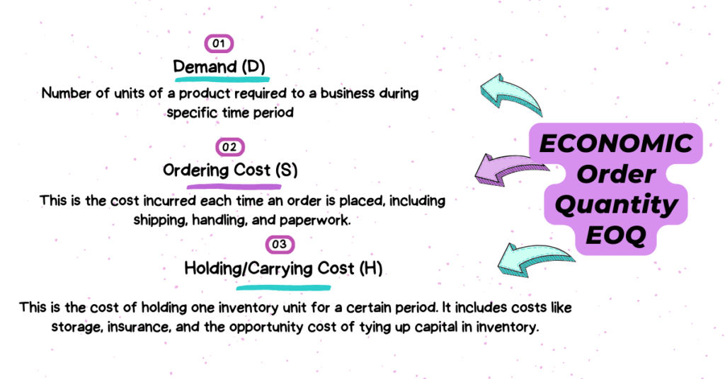
Demand (D): Number of units of a product required to a business during specific time period
Ordering Cost (S): This is the cost incurred each time an order is placed, including shipping, handling, and paperwork.
Holding Cost (H): This is the cost of holding one inventory unit for a certain period. It includes costs like storage, insurance, and the opportunity cost of tying up capital in inventory.

The Economic Order Quantity (EOQ) is a method that helps businesses determine the optimal order quantity to minimize the total cost of ordering and holding inventory. By utilizing the EOQ model, companies can find a balance between the costs associated with ordering too frequently (resulting in high ordering costs but low holding costs) and ordering in large quantities (resulting in low ordering costs but high holding costs). It is important to highlight that the EOQ model assumes a constant demand rate, no variability in lead time, and that all units ordered are received simultaneously. Although real-world conditions may differ, the EOQ model serves as a valuable starting point for making inventory management decisions.

Formula for Economic Order Quantity is:

$\mathbf{EOQ\ or\ Q = \ }\sqrt{\frac{\mathbf{2}\mathbf{DS}}{\mathbf{H}}}\$

Reorder Point/Ordering Point

The Reorder Point (ROP) is the inventory level at which a new order should be placed to replenish stock before it runs out. This takes into account the lead time required for the new stock to arrive. By considering the ROP, stockouts can be avoided during the time it takes to receive a new order.

Its formula is given below:

$\mathbf{Order\ Level = Maximum\ \ Consumption\ \times Lead\ Time})\textbf{Lead Time}$

Lead Time

Lead time plays a crucial role in material costing and inventory management as it determines the duration between placing an order and receiving the goods or materials from the supplier. This factor is essential in inventory planning and control as it ensures that the stock is available when required.

The lead time comprises two primary components, namely procurement or ordering time and delivery or transportation time. Procurement time involves the preparation and issuance of a purchase order, including activities such as order processing, paperwork, and communication. On the other hand, delivery time involves the shipping and delivery of the ordered goods, which includes transportation, handling, and any customs or regulatory procedures.

The sum of the procurement time and the delivery time results in the overall lead time. When establishing reorder points and order quantities, businesses must take into account the lead time to prevent stockouts and maintain a seamless inventory flow. In cases where the lead time is extended, it becomes essential to hold increased levels of safety stock to accommodate fluctuations in demand or disruptions in the supply chain.

Maximum Level of Inventory

The Maximum Level of Inventory, also referred to as the Maximum Stock Level or Maximum Level, represents the utmost quantity of inventory that a company is willing to maintain at any given point. Its purpose is to prevent unnecessary expenses linked to surplus inventory. It acts as a threshold, indicating that no further units should be ordered or produced until the inventory decreases. The determination of the Maximum Level takes into account several factors, including storage capacity, cash flow limitations, and the expenses incurred by holding excessive inventory.

Its formula is given below:

$\mathbf{Maximum\ Level = Order\ Level -}\left( \mathbf{Minimum\ Consumption\ during\ lead\ time} \right)\mathbf{+ EOQ}\$

Minimum Level of Inventory

The Minimum Level of Inventory, also referred to as the Minimum Stock Level or Safety Stock, denotes the smallest amount of inventory that a business is willing to maintain at any given point in time. This level is established as a precautionary measure to accommodate for uncertainties in both demand and supply. Its purpose is to ensure that there is always a minimum quantity of stock available to prevent stockouts during unforeseen fluctuations or delays in the supply chain. Determining the Minimum Level typically involves considering factors such as variations in demand, variability in lead time, and the potential consequences of running out of stock. It serves as a safety measure to provide a buffer against uncertainties and to uphold a certain level of service for customers.

Its formula is given below:

$\mathbf{Minimum\ Level = Order\ Level - (Average\ Consumption\ during\ lead\ time)}\$

Average Stock Level

The Average Stock Level, also referred to as the Average Level of Inventory, denotes the mean amount of inventory that a company holds during a particular timeframe. This metric is crucial in material costing and inventory management as it offers valuable information about the average capital invested in inventory.

Its formula is given below:

$\mathbf{Average\ Stock\ Level = Minimum\ Stock\ Level + \ }\frac{\mathbf{Reorder\ Quantity\ or\ EOQ}}{\mathbf{2}}\$

$\mathbf{Average\ Stock\ Level =}\frac{\mathbf{Reorder\ Quantity\ or\ EOQ}}{\mathbf{2}}\mathbf{+ Safety\ Stock}\$

Safety Stock

Safety Stock, on the other hand, is an additional quantity of inventory that is held to mitigate the risk of stockouts caused by uncertainties in demand or supply. It acts as a buffer to handle unexpected fluctuations in demand or delays in the supply chain.

Danger Level

The term “danger level” refers to a point where the inventory level is critically low and there is a high risk of stockouts, it could be similar to the reorder point or a situation where the safety stock has been depleted.

Its formula is given below:

$\mathbf{Danger\ Level = Average\ \ Consumption\ \times Time\ to\ get\ Emergency\ Supply}\$

Optimum number of Orders

The economic order quantity (EOQ) formula is utilized to determine the ideal order quantity that reduces the overall cost of holding and ordering inventory. By dividing the total demand for a specific period by the EOQ, one can obtain the optimal number of orders.

Its formula is given below:

$\mathbf{Optimum\ }\mathbf{Number\ of\ Orders\ Per\ Year =}\frac{\mathbf{Annual\ Requirement}}{\mathbf{EOQ}}\$

Order Frequency

Order frequency is simply a fraction of days in one year, and the number of orders per year. It simply tells the frequency of orders in a given year.

Its formula is given below:

$\mathbf{Frequency\ of\ Orders = \ }\frac{\mathbf{Number\ of\ Days\ in\ one\ year}}{\mathbf{Number\ of\ Orders\ Per\ year}}\$

Material Costing, Economic Order Quantity EOQ, Reorder Point/Ordering Point, Lead Time, Maximum Level of Inventory, Minimum Level of Inventory, Average Stock Level, Safety Stock, Danger Level, Optimum number of Orders, Order Frequency

Practical Example Questions for Understanding

Example Question 1

Question: Mashraq Industries has developed the following data to assist in controlling one of its inventory items. Economic Order Quantity 1000kg. Average Daily use 100 kg. Minimum Daily use 80 kg. Maximum daily use 120 kg Lead time 7 days.

Required:

Order point
Maximum inventory level
Minimum inventory level

Solution:

Data:

Economic Order Quantity EOQ =1000kg

Average Daily use = 100 kg

Minimum Daily use = 80 kg

Maximum daily use = 120 kg

Lead time = 7 days

$\left( \mathbf{a} \right)\mathbf{Order\ Level = Maximum\ \ Consumption\ \times Lead\ Time}\$

$\mathbf{Order\ Level = 120\ kg\ \times 7 = 840\ kg}\$

$\left( \mathbf{b} \right)\mathbf{Maximum\ Level = Order\ Level -}\left( \mathbf{Minimum\ Consumption\ during\ lead\ time} \right)\mathbf{+ EOQ}\$

$\mathbf{Maximum\ Level = 840 -}\left( \mathbf{80\ \times 7} \right)\mathbf{+ 1000 = 1280\ kg}\$

$\left( \mathbf{c} \right)\mathbf{Minimum\ Level = Order\ Level - (Average\ Consumption\ during\ lead\ time)}\$

$\mathbf{Minimum\ Level = 840 -}\left( \mathbf{100\ kg\ \times}\mathbf{7} \right)\mathbf{= 140\ kg}\$

Example Question 2

Question: Two types of materials A and B are used as follows:

Minimum usage: 20 units per week each

Normal usage: 40 units per week each.

Maximum usage: 60 units per week each.

Re-order Quantity (EOQ): A 400 units , B 600 units

Re-order period: A= 3 to 5 weeks, B=2 to 4 weeks

Calculate for two types of materials:

(a) Ordering point or re-order level

(b) Minimum level

(d) Average Stock level

Solution:

Data: Product A

Minimum usage: 20 units per week each

Normal usage: 40 units per week each.

Maximum usage: 60 units per week each.

Re-order Quantity (EOQ): A 400 units Re-order period: A= 3 to 5 weeks

$\left( \mathbf{a} \right)\mathbf{Order\ Level = Maximum\ \ Consumption\ \times Lead\ Time}\$

$\mathbf{Order\ Level = 60\ Units\ \times 5 = 300\ units}\$

$\left( \mathbf{b} \right)\mathbf{Minimum\ Level = Order\ Level - (Average\ Consumption\ during\ lead\ time)}\$

$\mathbf{Minimum\ Level = 300 -}\left( \mathbf{40\ Units\ \times}\frac{\mathbf{3 + 5}}{\mathbf{2}} \right)\mathbf{= 140\ units}\$

$\left( \mathbf{c} \right)\mathbf{Maximum\ Level = Order\ Level -}\left( \mathbf{Minimum\ Consumption\ during\ lead\ time} \right)\mathbf{+ EOQ}\$

$\mathbf{Maximum\ Level = 300 -}\left( \mathbf{20\ \times 3} \right)\mathbf{+ 400 = 640\ Units}\$

$\left( \mathbf{d} \right)\mathbf{Average\ Stock\ Level = Minimum\ Stock\ Level + \ }\frac{\mathbf{Reorder\ Quantity\ or\ EOQ}}{\mathbf{2}}\$

$\mathbf{Average\ Stock\ Level =}\frac{\mathbf{Reorder\ Quantity\ or\ EOQ}}{\mathbf{2}}\mathbf{+ Safety\ Stock}\$

$\mathbf{Average\ Stock\ Level = 140\ Units + \ }\frac{\mathbf{400}}{\mathbf{2}}\mathbf{= 340\ Units}\$

Data: Product B

Minimum usage: 20 units per week each

Normal usage: 40 units per week each.

Maximum usage: 60 units per week each.

Re-order Quantity (EOQ): B 600 units Re-order period: B= 2 to 4 weeks

$\left( \mathbf{a} \right)\mathbf{Order\ Level = Maximum\ \ Consumption\ \times Lead\ Time}\$

$\mathbf{Order\ Level = 60\ Units\ \times 4 = 240\ units}\$

$\left( \mathbf{b} \right)\mathbf{Minimum\ Level = Order\ Level - (Average\ Consumption\ during\ lead\ time)}\$

$\mathbf{Minimum\ Level = 240 -}\left( \mathbf{40\ Units\ \times}\frac{\mathbf{2 + 4}}{\mathbf{2}} \right)\mathbf{= 120\ units}\$

$\left( \mathbf{c} \right)\mathbf{Maximum\ Level = Order\ Level -}\left( \mathbf{Minimum\ Consumption\ during\ lead\ time} \right)\mathbf{+ EOQ}\$

$\mathbf{Maximum\ Level = 240 -}\left( \mathbf{20\ \times 2} \right)\mathbf{+ 600 = 800\ Units}\$

$\left( \mathbf{d} \right)\mathbf{Average\ Stock\ Level = Minimum\ Stock\ Level + \ }\frac{\mathbf{Reorder\ Quantity\ or\ EOQ}}{\mathbf{2}}\$

$\mathbf{Average\ Stock\ Level =}\frac{\mathbf{Reorder\ Quantity\ or\ EOQ}}{\mathbf{2}}\mathbf{+ Safety\ Stock}\$

$\mathbf{Average\ Stock\ Level = 120\ Units + \ }\frac{\mathbf{600}}{\mathbf{2}}\mathbf{= 420\ Units}\$

Example Question 3

Question: A manufacturing company estimates its carrying cost at 15% and ordering cost at Rs. 9 per order. The estimated annual requirement is 48,000 Units at a price of Rs. 4 per unit.

Required:

What is the most economical order quantity?
How many orders need to be placed?

Solution:

Data: Demand (D) = 48,000, Ordering Cost (S) = 9, Holding/Carrying Cost (H) = 15% of 4

$\left( \mathbf{a} \right)\mathbf{\ EOQor\ Q = \ }\sqrt{\frac{\mathbf{2}\mathbf{DS}}{\mathbf{H}}}\mathbf{=}\sqrt{\frac{\mathbf{2(48000)(9)}}{\mathbf{4(0.15)}}}\mathbf{=}\sqrt{\frac{\mathbf{864,000}}{\mathbf{0.60}}}\mathbf{=}\sqrt{\mathbf{14,40,000}}\mathbf{= 1200\ Units}\$

$\left( \mathbf{b} \right)\mathbf{Optimal\ Number\ of\ Orders\ Per\ Year =}\frac{\mathbf{D}}{\mathbf{Q}}\mathbf{=}\frac{\mathbf{48000}}{\mathbf{1200}}\mathbf{= 40}\$

Example Question 4

Question: Following estimates relate to material “Alpha”:

Requirement for six months 6000 units

Cost to place an order Rs. 10

Unit cost Rs. 4.80

Carrying cost 5%

Calculate economic order quantity.
Currently the company is purchasing this material in lots of 4,000 units. How much can the company save by buying in the most economical quantities?

Data:

$\mathbf{Demand\ (D)\ = \ 6000}\$

$\mathbf{Ordering\ Cost\ (S)\ = \ 10\ }\$

$\mathbf{Holding\ or\ Carrying\ Cost\ }\left( \mathbf{H} \right)\mathbf{= \ 0\ + \ }\left( \mathbf{5\%\ of\ 4.80} \right)\mathbf{= \ 0\ + \ 0.24\ = \ 0.24}\$

$\left( \mathbf{a} \right)\mathbf{\ EOQor\ Q = \ }\sqrt{\frac{\mathbf{2}\mathbf{DS}}{\mathbf{H}}}\mathbf{=}\sqrt{\frac{\mathbf{2(6000)(10)}}{\mathbf{0.24}}}\mathbf{=}\sqrt{\frac{\mathbf{120,000}}{\mathbf{0.24}}}\mathbf{=}\sqrt{\mathbf{500,000}}\mathbf{= 707\ Units}\$

(b)

			(a)		(b)	a +b
Annual Requirement	Order Size	No of Orders	Ordering Cost	Average Inventory	Carrying Cost	Total
6000	4000	1.5	15	2000	480	495
6000	707	8.486	84.86	353.5	84.84	169.7
Saving						325.3

Calculation

Formulas:

$\mathbf{Number\ of\ Orders = \ }\frac{\mathbf{Annual\ Requirement}}{\mathbf{Order\ SIze}}\$

$\mathbf{Ordering\ Cost = Number\ of\ Orders\ \times 10}\$

$\mathbf{Average\ Inventory = \ }\frac{\mathbf{Order\ Size}}{\mathbf{2}}\$

$\mathbf{Carrying\ Cost = Average\ Inventory\ \times 0.24}\$

Example Question 5

Question: Consumption forecast of a particular material is given here under:

Maximum daily consumption 600 units

Average daily consumption 500 units

Minimum daily consumption 400 units

Lead time 4 to 8 Days

Time to get emergency supplies 3 days

Economic order quantity 5000 Units

Required: Determine (a) Order level, (b) Minimum level, (c) Maximum level, (d) Danger level.

Solution:

$\left( \mathbf{a} \right)\mathbf{Order\ Level = Maximum\ \ Consumption\ \times Lead\ Time}\$

$\mathbf{Order\ Level = 600\ Units\ \times 8 = 4800\ Units}\$

$\left( \mathbf{b} \right)\mathbf{Minimum\ Level = Order\ Level - (Average\ Consumption\ during\ lead\ time)}\$

$\mathbf{Minimum\ Level = 4800 -}\left( \mathbf{500\ Units\ \times}\frac{\mathbf{4 + 8}}{\mathbf{2}} \right)\mathbf{= 1800}\$

$\left( \mathbf{c} \right)\mathbf{Maximum\ Level = Order\ Level -}\left( \mathbf{Minimum\ Consumption\ during\ lead\ time} \right)\mathbf{+ EOQ}\$

$\mathbf{Maximum\ Level = 4800 -}\left( \mathbf{400\ \times 4} \right)\mathbf{+ 5000 = 8200\ Units}\$

$\left( \mathbf{d} \right)\mathbf{Danger\ Level = Average\ Consumption\ during\ lead\ time\ for\ urgent\ supplies}\$

$\mathbf{Danger\ Level = Average\ \ Consumption\ \times Time\ to\ get\ Emergency\ Supply}\$

$\mathbf{Danger\ Level = 500\ \times 3 = 1500\ units}\$

Example Question 6

Question: A company purchases a certain material in lots of 900 units which is one quarter supply. The cost to place an order is Rs. 100 and carrying cost is 10%. The cost per unit of the material is Rs. 20.

Required:

(a) How much the company can save per year by following the Economic Order Quantity?

(b) Define lead time.

Solution:

Data:

Quarterly Requirement Material (D) = 900 Units

Ordering Cost (S) = 100

Carrying/Holding Cost (H) = 10% of 20 = 2

Per Unit Cost = Rs. 20

$\left( \mathbf{a} \right)\mathbf{\ EOQor\ Q = \ }\sqrt{\frac{\mathbf{2}\mathbf{DS}}{\mathbf{H}}}\mathbf{=}\sqrt{\frac{\mathbf{2(900)(100)}}{\mathbf{2}}}\mathbf{=}\sqrt{\frac{\mathbf{180,000}}{\mathbf{2}}}\mathbf{=}\sqrt{\mathbf{90,000}}\mathbf{= 300\ Units}\$

(b) Saving Computation, Assumed Annual Requirement is 900 x 4 = 3600 Units

			(a)		(b)	*a + b*
Annual Requirement	Order Size	No of Orders	Ordering Cost	Average Inventory	Carrying Cost	Total
3600	1800	2	200	900	1800	2000
3600	300	12	1200	150	300	1500
Saving						500

Computation

Formulas:

$\mathbf{Number\ of\ Orders = \ }\frac{\mathbf{Annual\ Requirement}}{\mathbf{Order\ SIze}}\$

$\mathbf{Ordering\ Cost = Number\ of\ Orders\ \times 100}\$

$\mathbf{Average\ Inventory = \ }\frac{\mathbf{Order\ Size}}{\mathbf{2}}\$

$\mathbf{Carrying\ Cost = Average\ Inventory\ \times 2}\$

Example Question 7

Question: Following data are available with respect to certain material:

Annual Requirement 56250 units

Cost to place an order Rs. 100

Annual Interest Rate 10%

Annual Carrying Cost per unit Rs. 5

Per Unit Cost Rs. 50

Required:

Economic Order Quantity
Number of Orders Per year
Frequency of Orders

Solution:

Data:

$\mathbf{Demand\ (D)\ = \ 56250}\$

$\mathbf{Ordering\ Cost\ (S)\ = \ 100\ }\$

$\mathbf{Holding/Carrying\ Cost\ (H)\ = \ 5\ + \ (10\%\ of\ 50)\ = \ 5\ + \ 5\ = \ 10}\$

$\left( \mathbf{a} \right)\mathbf{\ EOQor\ Q = \ }\sqrt{\frac{\mathbf{2}\mathbf{DS}}{\mathbf{H}}}\mathbf{=}\sqrt{\frac{\mathbf{2(56250)(100)}}{\mathbf{10}}}\mathbf{=}\sqrt{\frac{\mathbf{11,250,000}}{\mathbf{10}}}\mathbf{=}\sqrt{\mathbf{11,25,000}}\mathbf{= 1061\ Units}\$

$\left( \mathbf{b} \right)\mathbf{Number\ of\ Orders\ Per\ Year =}\frac{\mathbf{Annual\ Requirement}}{\mathbf{EOQ}}\$

$\mathbf{Number\ of\ Orders\ Per\ Year =}\frac{\mathbf{D}}{\mathbf{EOQ}}\mathbf{=}\frac{\mathbf{56250}}{\mathbf{1061}}\mathbf{= 53}\$

$\left( \mathbf{c} \right)\mathbf{Frequency\ of\ Orders = \ }\frac{\mathbf{Number\ of\ Days\ in\ one\ year}}{\mathbf{Number\ of\ Orders\ Per\ year}}\$

$\mathbf{Frequency\ of\ Orders = \ }\frac{\mathbf{360}}{\mathbf{53}}\mathbf{= 7}\$

Example Question 8

Question: The average daily requirement of 6″ diameter dish-shaped grinding wheel is 3 pieces. Time required to secure delivery from the usual supplier is 2 weeks. From the records of novelty Tools Works, it is found that maximum requirement of the wheel in any month of 4 weeks does not exceed 100 pieces and minimum requirement during any such period is not likely to fall below 50 pieces.

Required: You are asked to fix minimum and maximum limits and also the ordering level. Assume the economic order quantity to be 5 dozens. If 2 days are sufficient to receive emergency supply, fix also the danger level.

Solution:

Data:

Average Daily Requirement = 3 Pieces

Lead Time = 2 weeks

Maximum Requirement = 100 Pieces in 4 weeks

Weekly Maximum Requirement =

$\frac{100}{4} = 25\$