In this post, we are going to discuss, Statistics I HSSC I FBISE, Solved Paper 2008, MCQS, Short Questions, Extensive Questions. If you want to read the solved papers of Business Statistics ICOM II of FBISE, BISELHR, BISERWP and other boards, just explore the resource of the site. All the papers and reading resource including solved papers from intermediate, O, A level, graduation and masters level is given the website.
Table of Contents
Statistics I HSSC I FBISE, Solved Paper 2008, MCQS, Short Questions, Extensive Questions
Solved by Iftikhar Ali M.Sc. Economics, MCOM Finance Lecturer Statistics, Finance & Accounting
MCQS
| Q.1 Circle the Correct Option i.e. A/B/C/D. Each Part Carries 1 Mark. Bold options are Correct Answers | |||||
| (i) | What is the portion of the table containing the column captions called? | ||||
| A. Title | B. Boxhead | C. Stub | D. Body of the table | ||
| (ii) | What are the errors which tend to occur in the same direction called? | ||||
| A. Significant digits | B. Biased errors | C. Random errors | D. Chance errors | ||
| (iii) | Hourly temperature recorded by weather Bureau is an example of: | ||||
| A. Continuous & qualitative data | B. Continuous data | C. Discrete data | D. Qualitative data | ||
| (iv) | The data obtained from existing source is called. | ||||
| A. Discrete | B. Primary | C. Secondary | D. Continuous | ||
| (v) | Which of the following is the correct rounding off the number 4.003094 considering that it contains only three significant digits? | ||||
| A. 4.00 | B. 4.31 | C. 4.003 | D. 4.309 | ||
| (vi) | What is the classification said to be when data are arranged by their time of occurrence? | ||||
| A. Discrete | B. Geographical | C. Qualitative | D. Chronological | ||
| (vii) | A graph showing cumulative frequencies plotted against the upper class boundaries is called: | ||||
| A. Polygon | B. Barchart | C. Ogive | D. Frequency curve | ||
| (viii) | When X and Y are independent then Var (X-Y) is equal to: | ||||
| A. Var (X) — Var(Y) | B. Var(X)+Var(Y) | C. Var(X) + Var(-Y) | D. S.D(X) — S.D(Y) | ||
| (ix) | Where the link relatives are used? | ||||
| A. In fixed base method | B. In chain base method | C. In family budget method | D. In consumer’s price index number. | ||
| (x) | What is the sequence which follows random or irregular patterns of variation called? | ||||
| A. signal | B. Noise | C. Secular | D. Seasonal | ||
| (xi) | If r = 0.6, bxy = 1.2; what is the value of byx? | ||||
| A. 0.6 | B. 1.2 | C. 1.8 | D. 0.3 | ||
| (xii) | The best fitting trend is one for which sum of squares of residuals is: | ||||
| A. Zero | B. Least | C. Negative | D. Most | ||
| (xiii) | For what value of is the circular test for price index Number satisfied? | ||||
| A. | B. | C. | D. 1 | ||
| (xiv) | What kind of trend is the increased use of mobile phones in Pakistan? | ||||
| A. Secular | B. Seasonal | C. Cyclical | D. Irregular | ||
| (xv) | If we plot the paired observations (xi, yi) on a graph, what is the resulting set of points called? | ||||
| A. Ogive | B. Polygon | C. Histogram | D. Scatter diagram | ||
| (xvi) | The first moment X=0 of a distribution is 12.08. the mean is: | ||||
| A. 10.80 | B. 10.68 | C. 12.08 | D. 12.88 | ||
| (xvii) | For a symmetrical distribution: | ||||
| A. β1>0 | B. β1=0 | C. β1<0 | D. β1=3 | ||
Short Questions
SECTION-B
Q.2 Attempt any fourteen parts.
(i) Differentiate between diagrams and graphs. Write names of graphs of frequency distributions.
Answer:
- Frequency distribution can be shown in graphs but it cannot be shown in diagrams.
- Graphs are easy to make than diagrams.
- Only two variables can be used in graphs but in diagrams there may multi variables.
Different Frequency Distribution Graphs
- Histogram
- Frequency Polygon
- Ogive
- Bar Graph
- Pie Chart
- Pictogram
- Box and Whisker Plot
- Dot Plot
(ii) What are significant digits? How many significant digits are there in each of the following number?
149.8 (b) 0.00273 (c) 1.048905 (d) 80.00 (e) 0.95 (f) 0.09001
Answer:
Zeros appearing anywhere between two non-zero digits are significant. Example: 101.1203 has seven significant figures: 1, 0, 1, 1, 2, 0 and 3. Leading zeros are not significant. For example, 0.00052 has two significant figures: 5 and 2.
(Try)
(iii) A frequency table has four class intervals with 5, 9, 18, and 30 as frequencies in order. The left end point of third class interval and midpoint of fourth class interval are 20 and 35 respectively. Setup the frequency table and calculate arithmetic mean.
Solution
| Classes | Class Mark (X) | Frequency (f) |
| 5 | ||
| 9 | ||
| 20- | 18 | |
| 35 | 30 | |
| ∑f=62 |
| Classes | Class Mark (X) | Frequency (f) | fx |
| 0-10 | 5 | 5 | 25 |
| 10-20 | 15 | 9 | 135 |
| 20-30 | 25 | 18 | 450 |
| 30-40 | 35 | 30 | 1050 |
| ∑f=62 | ∑fx = 1660 |
(iv)The median, Upper and lower quartiles fourth and seventh deciles and fifteenth and 65th percentiles of a distribution of continuous variable were calculate as 63.94, 66.50, 73.67, 72.0, 60.93, 70.75 and 58.12. Identify the median, quartiles, deciles and percentiles.
Answer:
| Median | 1st Quartile | 3rd Quartile | 4th Decile | 7th Decile | 15th Percentile | 65th Percentile |
| 66.50 | 63.94 | 73.67 | 60.93 | 72 | 58.12 | 70.75 |
(v)The A.M of the series is 30.5 marks. Find the missing value.
| Marks | 10 | 20 | X | 40 | 50 |
| Frequency | 08 | 10 | 20 | 15 | 07 |
Solution
| Marks(X) | Frequency (f) | fx |
| 10 | 8 | 80 |
| 20 | 10 | 200 |
| X (30) Balancing Figure | 20 | 600 (Balancing Figure) |
| 40 | 15 | 600 |
| 50 | 7 | 350 |
![\[ \overline{\mathbf{X}}\mathbf{=}\frac{\mathbf{\sum}\mathbf{fx}}{\mathbf{\sum}\mathbf{f}}\ \]](https://bcfeducation.com/wp-content/ql-cache/quicklatex.com-3b45daacdea8872b882e83eede7d0359_l3.png "Rendered by QuickLaTeX.com")
![\[ \mathbf{30}\mathbf{.}\mathbf{5}\mathbf{=}\frac{\mathbf{\sum}\mathbf{fx}}{\mathbf{60}}\ \]](https://bcfeducation.com/wp-content/ql-cache/quicklatex.com-5191cbd59a7d01fbc9cb4d0bde6db441_l3.png "Rendered by QuickLaTeX.com")
![\[ \mathbf{\sum}\mathbf{fx}\mathbf{=}\mathbf{30}\mathbf{.}\mathbf{5x60}\mathbf{=}\mathbf{1830}\ \]](https://bcfeducation.com/wp-content/ql-cache/quicklatex.com-b5d6ec0ea1c2fee8928bc355421171b0_l3.png "Rendered by QuickLaTeX.com")
So the missing X is 30
(vi) Define absolute and relative measures of dispersion. Write the qualities of a good measure.
Answer:
Absolute measures of dispersion estimates the dispersion in absolute terms e.g. range, quartile deviation, mean deviation, standard deviation & variance are absolute measures of dispersion.
Relative measures of dispersion estimates the dispersion in relative terms e.g. coefficient of range, coefficient of quartile deviation, coefficient of mean deviation, coefficient of standard deviation & coefficient of variation are relative measures of dispersion.
Qualities of a Good Measure
Validity: Measure must be valid that means it must accurately measure the objective.
Easy to calculate: It must be easy to calculate.
Understandability: It must be easy to understand even for a common man.
Mathematical Formula: Is should has some mathematical formula.
Precision: A good measure should be precise for meaningful insight of the data and variables.
Represent Whole Data: All the data must be include in the calculation of the objective.
Independent to Extreme Values: It should not be affected from extreme values.
(vii) Calculate the mean and variance dispersion from the following data:
n=150, ∑(X-100) = 180, ∑(X-100)² = 245320
Solution
![\[ \mathbf{Mean}\overline{\mathbf{X}}\mathbf{=}\mathbf{A}\mathbf{+}\frac{\mathbf{\sum}\mathbf{d}}{\mathbf{n}}\mathbf{=}\mathbf{100}\mathbf{+}\frac{\mathbf{180}}{\mathbf{150}}\mathbf{=}\mathbf{101}\mathbf{.}\mathbf{2}\ \]](https://bcfeducation.com/wp-content/ql-cache/quicklatex.com-afb319c033cadad7b6080eae0dac2b3b_l3.png "Rendered by QuickLaTeX.com")
![\[ \mathbf{Variance}\mathbf{= \ }\frac{\mathbf{\sum}\mathbf{d}\mathbf{²}}{\mathbf{n}}\mathbf{-}\left( \frac{\mathbf{\sum}\mathbf{d}}{\mathbf{n}} \right)^{\mathbf{2}}\mathbf{=}\frac{\mathbf{245320}}{\mathbf{150}}\mathbf{-}\left( \frac{\mathbf{180}}{\mathbf{150}} \right)^{\mathbf{2}}\mathbf{=}\mathbf{1635}\mathbf{.}\mathbf{46 - 1}\mathbf{.}\mathbf{44}\mathbf{=}\mathbf{1634}\mathbf{.}\mathbf{02}\ \]](https://bcfeducation.com/wp-content/ql-cache/quicklatex.com-21d9ef3c3c46fc4da3294cd73106f5ec_l3.png "Rendered by QuickLaTeX.com")
(viii) In a certain distribution the first and second moments about the value 02 are -1 and 16 respectively. Find the mean and variance of the distribution. Also calculate coefficient of variation.
Solution:
![\[ \mathbf{m}\mathbf{1´ = - 1,\ m}\mathbf{2´ = 16}\ \]](https://bcfeducation.com/wp-content/ql-cache/quicklatex.com-9cc55dafc1e4e8f137a2186042c887d1_l3.png "Rendered by QuickLaTeX.com")
![\[ \mathbf{m}\mathbf{1´ =}\frac{\mathbf{\sum f(X - 2)}}{\mathbf{\sum f}}\mathbf{=}\frac{\mathbf{\sum fx}}{\mathbf{\sum f}}\mathbf{- 2}\frac{\mathbf{\sum f}}{\mathbf{\sum f}}\mathbf{=}\frac{\mathbf{\sum fx}}{\mathbf{\sum f}}\mathbf{- 2}\ \]](https://bcfeducation.com/wp-content/ql-cache/quicklatex.com-7300c5fcdf6341b1f63c1e0859b475ac_l3.png "Rendered by QuickLaTeX.com")
![\[ \mathbf{m}\mathbf{1´ =}\frac{\mathbf{\sum fx}}{\mathbf{\sum f}}\mathbf{- 2}\ \]](https://bcfeducation.com/wp-content/ql-cache/quicklatex.com-fa0bd70fdc34cb51a3e66fe8b4732f01_l3.png "Rendered by QuickLaTeX.com")
![\[ \mathbf{- 1 =}\overline{\mathbf{X}}\mathbf{- 2}\ \]](https://bcfeducation.com/wp-content/ql-cache/quicklatex.com-0eb9f74b3fdbca4baf3bbc4f28f7fd8c_l3.png "Rendered by QuickLaTeX.com")
![\[ \overline{\mathbf{X}}\mathbf{= - 1 + 2}\ \]](https://bcfeducation.com/wp-content/ql-cache/quicklatex.com-337f856fb9ef8e27a591857ad332c1da_l3.png "Rendered by QuickLaTeX.com")
![\[ \overline{\mathbf{X}}\mathbf{= 1}\ \]](https://bcfeducation.com/wp-content/ql-cache/quicklatex.com-15896d877ead64359d760ab35291323f_l3.png "Rendered by QuickLaTeX.com")
Moments about the mean are given by:
![\[ \mathbf{m}\mathbf{1 = 0}\ \]](https://bcfeducation.com/wp-content/ql-cache/quicklatex.com-7e64f22596748bc1225bc42d140f51b0_l3.png "Rendered by QuickLaTeX.com")
![\[ \mathbf{m}\mathbf{2 = m}\mathbf{2´ -}\left( \mathbf{m}\mathbf{1´} \right)^{\mathbf{2}}\ \]](https://bcfeducation.com/wp-content/ql-cache/quicklatex.com-9662e5a101ab9449edcf5027d0296044_l3.png "Rendered by QuickLaTeX.com")
![\[ \mathbf{m}\mathbf{2 = 16 -}\left( \mathbf{1} \right)^{\mathbf{2}}\mathbf{= 15 = Variance}\ \]](https://bcfeducation.com/wp-content/ql-cache/quicklatex.com-1b154d70d30fc65f981ffd619f6730a0_l3.png "Rendered by QuickLaTeX.com")
![\[ \mathbf{Variance = 15}\ \]](https://bcfeducation.com/wp-content/ql-cache/quicklatex.com-cd0169b4a1c3cb72393c9286515a22ec_l3.png "Rendered by QuickLaTeX.com")
![\[ \mathbf{Standard\ Deviation\ S.D =}\sqrt{\mathbf{Variance}}\mathbf{=}\sqrt{\mathbf{15}}\mathbf{= 3.872}\ \]](https://bcfeducation.com/wp-content/ql-cache/quicklatex.com-e3bf23b13253bed672e17dd3f3ed9083_l3.png "Rendered by QuickLaTeX.com")
![\[ \mathbf{C.V =}\frac{\mathbf{S.D}}{\mathbf{Mean}}\mathbf{\times 100}\ \]](https://bcfeducation.com/wp-content/ql-cache/quicklatex.com-9bf1b6cb80e00b136eced80f3ddbc7a7_l3.png "Rendered by QuickLaTeX.com")

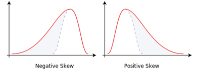
(ix) What would be the shape of frequency distribution if:
- Mean = Median = Mode
- Mean>Median>Mode
- Mean<Median<Mode
- Q3-Median>Median – Q1
Also Find Coefficient of range When Xm=100 & Xo=25
Solution
- Symmetrical data no skewness
- Positive skewness
- Negative skewness
- Moderately Positive Longer tail on right
![\[ \mathbf{CoefficientofRange}\mathbf{=}\frac{\mathbf{Xm - Xo}}{\mathbf{Xm}\mathbf{+}\mathbf{Xo}}\mathbf{= \ =}\frac{\mathbf{100 - 25}}{\mathbf{100}\mathbf{+}\mathbf{25}}\mathbf{= \ }\frac{\mathbf{75}}{\mathbf{125}}\mathbf{=}\mathbf{0}\mathbf{.}\mathbf{6}\mathbf{x}\mathbf{100}\mathbf{=}\mathbf{60}\mathbf{\%\ }\ \]](https://bcfeducation.com/wp-content/ql-cache/quicklatex.com-cc0fbfc281c8ef385bc7fe724b7b0446_l3.png "Rendered by QuickLaTeX.com")
(x) Distinguish between possitive and negative skewness with diagram.
Solution
(xi) What is consumer price index? How it is constructed?write the formula for each method.
Answer:
“Consumer Price Index numbers are intended to measure the changes in the prices paid by the consumer for purchasing a specified “basket” of goods and services during the current year as compared to the base year”.
Methods to Calculate
(i) Aggregative Expenditure Method
![\[ P_{0n} = \frac{\sum Pnqo}{\sum Poqo} \times 100\ \]](https://bcfeducation.com/wp-content/ql-cache/quicklatex.com-9166fd545cf4f59f67faeb648283d7d1_l3.png "Rendered by QuickLaTeX.com")
(ii) Household Budget method Or Family Budget Method
![\[ \mathbf{P}_{\mathbf{on}}\mathbf{=}\frac{\mathbf{\sum}\left( \frac{\mathbf{Pn}}{\mathbf{Po}} \right)\mathbf{Poqo}}{\mathbf{\sum Poqo}}\mathbf{\times 100 =}\frac{\mathbf{\sum IW}}{\mathbf{\sum W}}\ \]](https://bcfeducation.com/wp-content/ql-cache/quicklatex.com-6084156c4c39ae53ae7e5eca056f91cb_l3.png "Rendered by QuickLaTeX.com")
Where Price Relative =I =
![\[ \frac{\mathbf{Pn}}{\mathbf{Po}}\mathbf{\times 100}\mathbf{,\ W = Poqo}\ \]](https://bcfeducation.com/wp-content/ql-cache/quicklatex.com-fb5ccb559f8a2a0ce4a2c116636a1413_l3.png "Rendered by QuickLaTeX.com")
(xii) Distinguish between (a) simple linear and simple non linear regression (b) Perfectly positive and perfectly negative correlation.
Answer:
(a) A regression equation (or function) is linear when it is linear in the parameters whereas it is non-linear when it is non-linear in parameter.
(b) If one variable increases and another also increases with equal proportion or vice-versa then the relationship is perfectly positive in correlation and its answer always be +1.
If one variable increases and another decreases with equal proportion or vice-versa then the relationship is perfectly negative in correlation and its answer always be -1.
(xiii) Determine the estimated regression equation:
![\[ \widehat{\mathbf{y}}\mathbf{\ = \ a\ + \ bx\ if:}\ \]](https://bcfeducation.com/wp-content/ql-cache/quicklatex.com-c446d54ba28b07cc990f2f88cf8e2ea5_l3.png "Rendered by QuickLaTeX.com")
(a)
![\[ \mathbf{n\ = \ 10,\ \sum x\ = \ 20,\ \sum y\ = \ 260,\ \sum x²\ = \ 3144,\ \sum xy\ = \ 1500}\ \]](https://bcfeducation.com/wp-content/ql-cache/quicklatex.com-93509db8fcbdcbb8d7ebb5d721662353_l3.png "Rendered by QuickLaTeX.com")
(b)
![\[ \mathbf{n\ = \ 7,\ \sum x\ = \ 0,\ \sum y\ = \ 245,\ \sum x²\ = \ 28,\ \sum xy\ = \ 2000}\ \]](https://bcfeducation.com/wp-content/ql-cache/quicklatex.com-86e01fffb98c91753e9c1607c9d6a2df_l3.png "Rendered by QuickLaTeX.com")
Solution (a)
![\[ \mathbf{a}\mathbf{=}\overline{\mathbf{y}}\mathbf{- b}\overline{\mathbf{X}}\ \]](https://bcfeducation.com/wp-content/ql-cache/quicklatex.com-ce6d2ee229e792c56e2eaa9808fe5abc_l3.png "Rendered by QuickLaTeX.com")
![\[ \mathbf{b}\mathbf{= \ }\frac{\mathbf{\sum}\mathbf{xy - n}\overline{\mathbf{X}}\overline{\mathbf{Y}}}{\mathbf{\sum}\mathbf{X}^{\mathbf{2}}\mathbf{- n}\mathbf{(}\overline{\mathbf{X}}\mathbf{)}\mathbf{²}}\ \]](https://bcfeducation.com/wp-content/ql-cache/quicklatex.com-3625f18faa24300402ae4529823b026d_l3.png "Rendered by QuickLaTeX.com")
![\[ \mathbf{Mean}\overline{\mathbf{X}}\mathbf{=}\frac{\mathbf{\sum}\mathbf{X}}{\mathbf{n}}\mathbf{=}\frac{\mathbf{20}}{\mathbf{10}}\mathbf{=}\mathbf{2}\mathbf{,\ }\mathbf{Mean}\overline{\mathbf{Y}}\mathbf{=}\frac{\mathbf{\sum}\mathbf{Y}}{\mathbf{n}}\mathbf{=}\frac{\mathbf{260}}{\mathbf{10}}\mathbf{=}\mathbf{26}\ \]](https://bcfeducation.com/wp-content/ql-cache/quicklatex.com-6ecb63c829bc44df1963e5178e6d3250_l3.png "Rendered by QuickLaTeX.com")
![\[ \mathbf{b}\mathbf{= \ }\frac{\mathbf{\sum}\mathbf{xy - n}\overline{\mathbf{X}}\overline{\mathbf{Y}}}{\mathbf{\sum}\mathbf{X}^{\mathbf{2}}\mathbf{- n}\mathbf{(}\overline{\mathbf{X}}\mathbf{)}\mathbf{²}}\mathbf{= \ }\frac{\mathbf{1500 -}\left( \mathbf{10} \right)\left( \mathbf{2} \right)\mathbf{(}\mathbf{26}\mathbf{)}}{\mathbf{3144 - 10}\mathbf{(}\mathbf{2}\mathbf{)}\mathbf{²}}\mathbf{= \ }\frac{\mathbf{980}}{\mathbf{3104}}\mathbf{=}\mathbf{0}\mathbf{.}\mathbf{315}\ \]](https://bcfeducation.com/wp-content/ql-cache/quicklatex.com-1179d727e8a56a0727cbcaa85188644b_l3.png "Rendered by QuickLaTeX.com")
![\[ \mathbf{a}\mathbf{=}\mathbf{26 -}\left( \mathbf{0}\mathbf{.}\mathbf{315} \right)\left( \mathbf{2} \right)\mathbf{= \ }\mathbf{25}\mathbf{.}\mathbf{37}\ \]](https://bcfeducation.com/wp-content/ql-cache/quicklatex.com-31328bb2c061de219a250ed9be274917_l3.png "Rendered by QuickLaTeX.com")
![\[ \widehat{\mathbf{y}}\mathbf{\ = \ a\ + \ bx\ = \ y\hat{}\ = \ 25.37\ + \ 0.315}\mathbf{x}\ \]](https://bcfeducation.com/wp-content/ql-cache/quicklatex.com-cd1db754aa686a284b5dfc1686beadfe_l3.png "Rendered by QuickLaTeX.com")
Solution (b)
![\[ \mathbf{Mean}\overline{\mathbf{X}}\mathbf{=}\frac{\mathbf{\sum}\mathbf{X}}{\mathbf{n}}\mathbf{=}\frac{\mathbf{0}}{\mathbf{7}}\mathbf{=}\mathbf{0}\mathbf{,\ }\mathbf{Mean}\overline{\mathbf{Y}}\mathbf{=}\frac{\mathbf{\sum}\mathbf{Y}}{\mathbf{n}}\mathbf{=}\frac{\mathbf{245}}{\mathbf{7}}\mathbf{=}\mathbf{35}\ \]](https://bcfeducation.com/wp-content/ql-cache/quicklatex.com-0f06ca09e154b7db11d9df10b980b4d8_l3.png "Rendered by QuickLaTeX.com")
![\[ \mathbf{b}\mathbf{= \ }\frac{\mathbf{\sum}\mathbf{xy - n}\overline{\mathbf{X}}\overline{\mathbf{Y}}}{\mathbf{\sum}\mathbf{X}^{\mathbf{2}}\mathbf{- n}\left( \overline{\mathbf{X}} \right)^{\mathbf{2}}}\mathbf{= \ }\frac{\mathbf{2000 -}\left( \mathbf{7} \right)\left( \mathbf{0} \right)\left( \mathbf{35} \right)}{\mathbf{28 - 7}\left( \mathbf{0} \right)^{\mathbf{2}}}\mathbf{= \ }\frac{\mathbf{1755}}{\mathbf{28}}\mathbf{=}\mathbf{62.67}\ \]](https://bcfeducation.com/wp-content/ql-cache/quicklatex.com-91affb9760829f784a5416b68183b264_l3.png "Rendered by QuickLaTeX.com")
![\[ \mathbf{a}\mathbf{=}\mathbf{35 -}\left( \mathbf{62.67} \right)\left( \mathbf{0} \right)\mathbf{= \ }\mathbf{35}\ \]](https://bcfeducation.com/wp-content/ql-cache/quicklatex.com-5ab6510ce55e44ee542eca6ddba96cfe_l3.png "Rendered by QuickLaTeX.com")
![\[ \widehat{\mathbf{y}}\mathbf{\ = \ a\ + \ bx\ }\ \]](https://bcfeducation.com/wp-content/ql-cache/quicklatex.com-5d7cfb6b5b544f2501560a245660f47f_l3.png "Rendered by QuickLaTeX.com")
![\[ \widehat{\mathbf{y}}\mathbf{= 35\ + \ 62.67}\mathbf{x\ \ }\ \]](https://bcfeducation.com/wp-content/ql-cache/quicklatex.com-eebbf4ca1ea6749c3e9404b0146cdb41_l3.png "Rendered by QuickLaTeX.com")
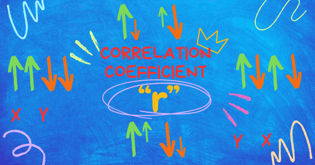
(xiv) What inference would you draw if correlation coefficient is? (a) +1 (b) -1 (c) 0 (d) -0.98 (e) 0.2 (f) 2
Answer:
(a) Perfectly positive
(b) Perfectly Negative
(c) Negative
(d) Positive
(e) Not Possible
(xv) Find the correlation coefficient from the regression coefficients. (a) 1.2 & 0.6 (b) -0.76 and -0.82 (c) -1.6 and -0.4
Solution
(a) 
(b) 
(c) 
(xvi) Differentiate between signal and noise. Write the additive model of the time series.
Answer:
Statistical signal: In Time Series analysis, Signal is a pattern of regular variation. It provides the meaningful insight of the data that express the genuine change or variation over the period of time.
Statistical noise: In Time Series Analysis, it represents the irregular, random variations of the data over the period of time. These random fluctuations or noise may be caused by errors, external factors. It is simply the disturbance of the data which is unpredictable.
Additive Model
A common approach to modeling time–series data (Y) in which it is assumed that the four components of a time series; trend component (T), seasonal component (S), cyclical component (C) and irregular component (I), are added to form the values of the time series at each time period.
Y = T + S + C + I
(xvii) Describe the merits and demerits of free hand, semi average and moving average method. Illustrate each method with example.
Answer:
Merits & Demerits of Free hand Curve Method
Merits :
- It is very simplest method for study trend values and easy to draw trend.
- Sometimes the trend line drawn by the statistician experienced in computing trend may be considered better than a trend line fitted by the use of a mathematical formula.
- Although the free hand curves method is not recommended for beginners, it has considerable merits in the hands of experienced statisticians and widely used in applied situations.
Demerits:
- This method is highly subjective and curve varies from person to person who draws it.
- The work must be handled by skilled and experienced people.
- Since the method is subjective, the prediction may not be reliable.
- While drawing a trend line through this method a careful job has to be done.
Merits & Demerits of Semi-Average
Merits:
- This method is simple to understand as compare to moving average method and method of least squares.
- This is an objective method of measuring trend as everyone who applies this method is bound to get the same result.
Demerits:
- The method assumes straight line relationship between the plotted points regardless of the fact whether that relationship exists or not.
- The main drawback of this method is if we add some more data to the original data then whole calculation is to be done again for the new data to get the trend values and the trend line also changes.
- As the A.M of each half is calculated, an extreme value in any half will greatly affect the points and hence trend calculated through these points may not be precise enough for forecasting the future.
Merits & Demerits of Moving-Average
Merits:
- This method is simple to understand and easy to execute.
- It has the flexibility in application in the sense that if we add data for a few more time periods to the original data, the previous calculations are not affected and we get a few more trend values.
- It gives a correct picture of the long term trend if the trend is linear.
- If the period of moving average coincides with the period of oscillation (cycle), the periodic fluctuations are eliminated.
- The moving average has the advantage that it follows the general movements of the data and that its shape is determined by the data rather than the statistician’s choice of mathematical function.
Demerits:
- For a moving average of 2m+1, one does not get trend values for first m and last m periods.
- As the trend path does not correspond to any mathematical; function, it cannot be used for forecasting or predicting values for future periods.
- If the trend is not linear, the trend values calculated through moving averages may not show the true tendency of data.
- The choice of the period is sometimes left to the human judgment and hence may carry the affect of human bias.
(xviii) (a) The semi averages for 1964-1972 (both inclusive) are 82.5 and 104. Find the trend values. (b) 15 observations from 1986 to 2000 on real net sales is (1986 as base year). What is the fitted trend value for this time series on real net sales for the 5th year?
Solution
| Time | Average | Trends |
| 1964 | 82.5 | 77.125 – 5.375 = 71.75 |
| 1965 | 82.5 – 5.375 = 77.125 | |
| 1966 | 87.875 – 5.375 = 82.5 | |
| 1967 | 82.5 +5.375 = 87.875 | |
| 1968 | 87.875 + 5.375 =93.25 | |
| 1969 | 104 | 93.25 + 5.375 = 98.625 |
| 1970 | 98.625 + 5.375 = 104 | |
| 1971 | 104 + 5.375 = 109.375 | |
| 1972 | 109.375 + 5.375 = 114.75 |
![\[ \mathbf{Calculation\ of\ Trend\ =}\frac{\mathbf{104\ -\ 82.5}}{\mathbf{4}}\mathbf{\ = \ 5.375\ }\ \]](https://bcfeducation.com/wp-content/ql-cache/quicklatex.com-1050c15ae70294969dfffaa645eedf18_l3.png "Rendered by QuickLaTeX.com")
![\[ \left( \mathbf{b} \right)\widehat{\mathbf{y}}\mathbf{\ = \ 2.4\ + \ 0.5}\mathbf{X}\ \]](https://bcfeducation.com/wp-content/ql-cache/quicklatex.com-511deb68af26099cbd6818d737a26f79_l3.png "Rendered by QuickLaTeX.com")
![\[ \widehat{\mathbf{y}}\mathbf{\ = \ 2.4\ + \ 0.5(5)\ = \ 4.9}\ \]](https://bcfeducation.com/wp-content/ql-cache/quicklatex.com-6b46aa60c695aaf3dec0328163b01b46_l3.png "Rendered by QuickLaTeX.com")
Extensive Questions
Section C
Q.3 Calculate the first four moments about the value 7.95 and then the moments about the mean. Also calculate b2. Is the distribution normal?
| Group | Frequency | Group | Frequency |
| 3.5-4.4 | 5 | 8.5-9.4 | 11 |
| 4.5-5.4 | 10 | 9.5-10.4 | 10 |
| 5.5-6.4 | 13 | 10.5-11.4 | 4 |
| 6.5-7.4 | 17 | 11.5-12.4 | 1 |
| 7.5-8.4 | 29 |
Solution:
| Classes | f | fx | D = X – 7.95 | fD | | | |
| 3.5-4.4 | 5 | 3.95 | -4 | -20 | 80 | -320 | 1280 |
| 4.5-5.4 | 10 | 4.95 | -3 | -30 | 90 | -270 | 810 |
| 5.5-6.4 | 13 | 5.95 | -2 | -26 | 52 | -104 | 208 |
| 6.5-7.4 | 17 | 6.95 | -1 | -17 | 17 | -17 | 17 |
| 7.5-8.4 | 29 | 7.95 | 0 | 0 | 0 | 0 | 0 |
| 8.5-9.4 | 11 | 8.95 | 1 | 11 | 11 | 11 | 11 |
| 9.5-10.4 | 10 | 9.95 | 2 | 20 | 40 | 80 | 160 |
| 10.5-11.4 | 4 | 10.95 | 3 | 12 | 36 | 108 | 324 |
| 11.5-12.4 | 1 | 11.95 | 4 | 4 | 16 | 64 | 256 |
| 100 | -46 | 342 | -448 | 3066 | |||
| | | | |
![\[ fD^2 \]](https://bcfeducation.com/wp-content/ql-cache/quicklatex.com-9108314f64b426e1b1f963ffe08c892a_l3.png "Rendered by QuickLaTeX.com")
![\[ fD^3 \]](https://bcfeducation.com/wp-content/ql-cache/quicklatex.com-d78e03eef581a4ae53caa70f03f1b8f9_l3.png "Rendered by QuickLaTeX.com")
![\[ fD^4 \]](https://bcfeducation.com/wp-content/ql-cache/quicklatex.com-505c4d12fdae3fc36e16580f3ea1138e_l3.png "Rendered by QuickLaTeX.com")
![\[ \sum f= \]](https://bcfeducation.com/wp-content/ql-cache/quicklatex.com-a95d1a7786772792cd12e523a796c827_l3.png "Rendered by QuickLaTeX.com")
![\[ \sum fD= \]](https://bcfeducation.com/wp-content/ql-cache/quicklatex.com-1bbdbf2241c7657b34f8074198bc6715_l3.png "Rendered by QuickLaTeX.com")
![\[ \sum fD^2= \]](https://bcfeducation.com/wp-content/ql-cache/quicklatex.com-8406035accb657374f649300f025c8c3_l3.png "Rendered by QuickLaTeX.com")
![\[ \sum fD^3= \]](https://bcfeducation.com/wp-content/ql-cache/quicklatex.com-24aae84f788ad640665907c795e88344_l3.png "Rendered by QuickLaTeX.com")
![\[ \sum fD^4= \]](https://bcfeducation.com/wp-content/ql-cache/quicklatex.com-06710edb1abd7ac1934e2be0dd264295_l3.png "Rendered by QuickLaTeX.com")
Moments about X = 7.95
![\[ \mathbf{m}\mathbf{1´ =}\frac{\mathbf{\sum fD}}{\mathbf{\sum f}}\mathbf{=}\frac{\mathbf{- 46}}{\mathbf{100}}\mathbf{= - 0.46}\ \]](https://bcfeducation.com/wp-content/ql-cache/quicklatex.com-008b0c624bdbfb7a847ac2cd9fe7c6f8_l3.png "Rendered by QuickLaTeX.com")
![\[ \mathbf{m}\mathbf{2´ =}\frac{\mathbf{\sum f}\mathbf{D}^{\mathbf{2}}}{\mathbf{\sum f}}\mathbf{=}\frac{\mathbf{342}}{\mathbf{100}}\mathbf{= 3.42}\ \]](https://bcfeducation.com/wp-content/ql-cache/quicklatex.com-6b703e42c478e033100af1c614394597_l3.png "Rendered by QuickLaTeX.com")
![\[ \mathbf{m}\mathbf{3´ =}\frac{\mathbf{\sum f}\mathbf{D}^{\mathbf{3}}}{\mathbf{\sum f}}\mathbf{=}\frac{\mathbf{- 448}}{\mathbf{100}}\mathbf{= - 4.48}\ \]](https://bcfeducation.com/wp-content/ql-cache/quicklatex.com-8af8c05364457f809db986497da49732_l3.png "Rendered by QuickLaTeX.com")
![\[ \mathbf{m}\mathbf{4´ =}\frac{\mathbf{\sum f}\mathbf{D}^{\mathbf{4}}}{\mathbf{\sum f}}\mathbf{=}\frac{\mathbf{3066}}{\mathbf{100}}\mathbf{= 30.66}\ \]](https://bcfeducation.com/wp-content/ql-cache/quicklatex.com-da14caecfa38d89326b34504166238ac_l3.png "Rendered by QuickLaTeX.com")
Moments about A.M are:
![\[ \mathbf{m}\mathbf{2 = 3.42 -}\left( \mathbf{- 0.46} \right)^{\mathbf{2}}\mathbf{= 3.2084}\ \]](https://bcfeducation.com/wp-content/ql-cache/quicklatex.com-23ef48df50eb07574d357471cb0fc2d3_l3.png "Rendered by QuickLaTeX.com")
![\[ \mathbf{m}\mathbf{3 = m}\mathbf{3´ - 3}\mathbf{m}\mathbf{1´m}\mathbf{2´ + 2}\left( \mathbf{m}\mathbf{1´} \right)^{\mathbf{3}}\ \]](https://bcfeducation.com/wp-content/ql-cache/quicklatex.com-0a2938e58fe1d92535492202464daecf_l3.png "Rendered by QuickLaTeX.com")
![\[ \mathbf{m}\mathbf{3 = - 4.48 - 3( - 0.46)(3.42) + 2}\left( \mathbf{- 0.46} \right)^{\mathbf{3}}\ \]](https://bcfeducation.com/wp-content/ql-cache/quicklatex.com-a419e1b779768d6dd34499d3b7a38655_l3.png "Rendered by QuickLaTeX.com")
![\[ \mathbf{m}\mathbf{3 = - 4.48 + 4.7196 - 0.194672}\ \]](https://bcfeducation.com/wp-content/ql-cache/quicklatex.com-92ffbcfb5820a5a8f84009715ac27d54_l3.png "Rendered by QuickLaTeX.com")
![\[ \mathbf{m}\mathbf{3 = 0.044928}\ \]](https://bcfeducation.com/wp-content/ql-cache/quicklatex.com-662162258324ce4185d137ff2eee1d06_l3.png "Rendered by QuickLaTeX.com")
![\[ \mathbf{m}\mathbf{4 = m}\mathbf{4´ - 4}\mathbf{m}\mathbf{1´m}\mathbf{3´ + 6}\left( \mathbf{m}\mathbf{1´} \right)^{\mathbf{2}}\mathbf{m}\mathbf{2´ - 3}\left( \mathbf{m}\mathbf{1´} \right)^{\mathbf{4}}\ \]](https://bcfeducation.com/wp-content/ql-cache/quicklatex.com-e40b94380f691304bd16d9490662e485_l3.png "Rendered by QuickLaTeX.com")
![\[ \mathbf{m}\mathbf{4 = 30.66 - 4( - 0.46)( - 4.48) + 6}\left( \mathbf{- 0.46} \right)^{\mathbf{2}}\mathbf{(3.42) - 3}\left( \mathbf{- 0.46} \right)^{\mathbf{4}}\ \]](https://bcfeducation.com/wp-content/ql-cache/quicklatex.com-6c27fba955df71a2a5f281819cb7c48f_l3.png "Rendered by QuickLaTeX.com")
![\[ \mathbf{m}\mathbf{4 = 30.66 - 8.2432 + 4.3420 - 0.134323}\ \]](https://bcfeducation.com/wp-content/ql-cache/quicklatex.com-032c013de60bb31756aa4c7da2ccdbaf_l3.png "Rendered by QuickLaTeX.com")
![\[ \mathbf{m}\mathbf{4 = 26.6244}\ \]](https://bcfeducation.com/wp-content/ql-cache/quicklatex.com-edb41a5894d6d7578c2014b099a4fa17_l3.png "Rendered by QuickLaTeX.com")
![\[ \mathbf{b}_{\mathbf{2}}\mathbf{=}\frac{\mathbf{m}\mathbf{4}}{\mathbf{m}\mathbf{2}^{\mathbf{2}}}\mathbf{=}\frac{\mathbf{26.6244}}{\left( \mathbf{3.2084} \right)^{\mathbf{2}}}\mathbf{=}\frac{\mathbf{26.6244}}{\mathbf{10.2938}}\mathbf{= 2.586}\ \]](https://bcfeducation.com/wp-content/ql-cache/quicklatex.com-cafe8b54ca9619798a01e454fddecc42_l3.png "Rendered by QuickLaTeX.com")
Q.4 Calculate base year weighted and current year weighted index number from the following data. Also calculate Fisher’s Index number:
| Items | Base Year | Current year | ||
| Price | Quantity | Price | Quantity | |
| A | 03 | 70 | 04 | 75 |
| B | 05 | 80 | 06 | 90 |
| C | 08 | 40 | 10 | 55 |
| D | 10 | 50 | 12 | 60 |
Solution:
| Article | Base Year | Current Year | ||||||
| Price (Po) | Quantity (qo) | Price (P1) | Quantity (q1) | poqo | p1qo | p1q1 | poq1 | |
| A | 3 | 70 | 4 | 75 | 210 | 280 | 300 | 225 |
| B | 5 | 80 | 6 | 90 | 400 | 480 | 540 | 450 |
| C | 8 | 40 | 10 | 55 | 320 | 400 | 550 | 440 |
| D | 10 | 50 | 12 | 60 | 500 | 600 | 720 | 600 |
| Sum | 1430 | 1760 | 2110 | 1715 | ||||
| ∑poqo = | ∑p1qo = | ∑p1q1 = | ∑poq1 = | |||||
![\[ \left( \mathbf{i} \right)\mathbf{Base\ year\ weighted}\mathbf{\ }\mathbf{Index}\mathbf{\ 2000}\mathbf{=}\frac{\mathbf{\sum}\mathbf{p}_{\mathbf{1}}\mathbf{q}_{\mathbf{0}}}{\mathbf{\sum}\mathbf{p}_{\mathbf{0}}\mathbf{q}_{\mathbf{0}}}\mathbf{x\ 100}\ \]](https://bcfeducation.com/wp-content/ql-cache/quicklatex.com-3fcbf8190c37fc435bbaddfb85ff8cfa_l3.png "Rendered by QuickLaTeX.com")
![\[ \mathbf{Base\ year\ weighted}\mathbf{\ }\mathbf{Index}\mathbf{=}\frac{\mathbf{1760}}{\mathbf{1430}}\mathbf{\ \times \ 100 = \ 123.07}\ \]](https://bcfeducation.com/wp-content/ql-cache/quicklatex.com-b0b4fa0a31dd60856460656800a52ce9_l3.png "Rendered by QuickLaTeX.com")
![\[ \left( \mathbf{ii} \right)\mathbf{Current\ year\ weighted}\mathbf{\ }\mathbf{Index}\mathbf{\ 2000}\mathbf{=}\frac{\mathbf{\sum}\mathbf{p}_{\mathbf{1}}\mathbf{q}_{\mathbf{1}}}{\mathbf{\sum}\mathbf{p}_{\mathbf{0}}\mathbf{q}_{\mathbf{1}}}\mathbf{x\ 100}\ \]](https://bcfeducation.com/wp-content/ql-cache/quicklatex.com-4ba12a462bdd646da47f3411e1268a40_l3.png "Rendered by QuickLaTeX.com")
![\[ \mathbf{Current\ year\ weighted}\mathbf{\ }\mathbf{Index}\mathbf{\ }\mathbf{\ }\mathbf{=}\frac{\mathbf{2110}}{\mathbf{1715}}\mathbf{\times \ 100 = 123.03}\ \]](https://bcfeducation.com/wp-content/ql-cache/quicklatex.com-cf8796d4accd36be0f720ae573b4b4c0_l3.png "Rendered by QuickLaTeX.com")
![\[ \left( \mathbf{iii} \right)\mathbf{Fishe}\mathbf{r}^{\mathbf{'}}\mathbf{s\ Ideal\ Index}\mathbf{\ }\mathbf{=}\sqrt{\mathbf{L \times P}}\ \]](https://bcfeducation.com/wp-content/ql-cache/quicklatex.com-3d89576f786bfcb3b84351bd5227631c_l3.png "Rendered by QuickLaTeX.com")
![\[ \mathbf{Fishe}\mathbf{r}^{\mathbf{'}}\mathbf{s\ Ideal\ Index}\mathbf{\ }\mathbf{=}\sqrt{\mathbf{123.07 \times 123.03}}\ \]](https://bcfeducation.com/wp-content/ql-cache/quicklatex.com-ec7719746353e86b17c04c2bb1663393_l3.png "Rendered by QuickLaTeX.com")
![\[ \mathbf{Fishe}\mathbf{r}^{\mathbf{'}}\mathbf{s\ Ideal\ Index}\mathbf{\ }\mathbf{= 123.04}\ \]](https://bcfeducation.com/wp-content/ql-cache/quicklatex.com-4444e75ee50c91d92203e46857105f07_l3.png "Rendered by QuickLaTeX.com")
Q.5 The marks obtained by 10 students in December test (X) and promotion test (Y) are given below:
(i) Estimate the marks in the promotion test (Y) if a student who was sick obtained 60 marks in the December test (X)
(ii) If a student who migrated after the december test obtained 75 marks in the promotion test (Y), estimate his marks in the december test (X) had he been admitted earlier.
| Students | X | Y |
| 01 | 41 | 60 |
| 02 | 45 | 63 |
| 03 | 50 | 60 |
| 04 | 68 | 48 |
| 05 | 47 | 85 |
| 06 | 77 | 56 |
| 07 | 90 | 53 |
| 08 | 100 | 97 |
| 09 | 80 | 74 |
| 10 | 100 | 98 |
Solution:
| X | Y | XY | | |
| 41 | 60 | 2460 | 1681 | 3600 |
| 45 | 63 | 2835 | 2025 | 3969 |
| 50 | 60 | 3000 | 2500 | 3600 |
| 68 | 48 | 3264 | 4624 | 2304 |
| 47 | 85 | 3995 | 2209 | 7225 |
| 77 | 56 | 4312 | 5929 | 3136 |
| 90 | 53 | 4770 | 8100 | 2809 |
| 100 | 97 | 9700 | 10000 | 9409 |
| 80 | 74 | 5920 | 6400 | 5476 |
| 100 | 98 | 9800 | 10000 | 9604 |
| 698 | 694 | 50056 | 53468 | 51132 |
| | | | |
![\[ X^2 \]](https://bcfeducation.com/wp-content/ql-cache/quicklatex.com-5f8b829c6415b114cdcd6b73d7e884d6_l3.png "Rendered by QuickLaTeX.com")
![\[ Y^2 \]](https://bcfeducation.com/wp-content/ql-cache/quicklatex.com-7a7a22947fa626aa5e6486b35ed5c265_l3.png "Rendered by QuickLaTeX.com")
![\[ \sum X =\ \]](https://bcfeducation.com/wp-content/ql-cache/quicklatex.com-549eb0233f13035f3abc11b081fedbaf_l3.png "Rendered by QuickLaTeX.com")
![\[ \sum Y =\ \]](https://bcfeducation.com/wp-content/ql-cache/quicklatex.com-182ffb8af128b0843d0c78ea4f4faea6_l3.png "Rendered by QuickLaTeX.com")
![\[ \sum XY =\ \]](https://bcfeducation.com/wp-content/ql-cache/quicklatex.com-b955b1f52add4baaddd786f683c42be8_l3.png "Rendered by QuickLaTeX.com")
![\[ \sum X^{2} =\ \]](https://bcfeducation.com/wp-content/ql-cache/quicklatex.com-56900a1443801f465600cef982c970cd_l3.png "Rendered by QuickLaTeX.com")
![\[ \sum Y^{2} =\ \]](https://bcfeducation.com/wp-content/ql-cache/quicklatex.com-46c5b3477f95cf4a7fac3172df3ea8d2_l3.png "Rendered by QuickLaTeX.com")
Regression Equation Y on X
![\[ \widehat{\mathbf{y}}\mathbf{\ = \ a\ + \ bx}\ \]](https://bcfeducation.com/wp-content/ql-cache/quicklatex.com-3901a71864808555e95727411313ea62_l3.png "Rendered by QuickLaTeX.com")
![\[ \mathbf{Mean}\overline{\mathbf{X}}\mathbf{=}\frac{\mathbf{\sum}\mathbf{X}}{\mathbf{n}}\mathbf{=}\frac{\mathbf{698}}{\mathbf{10}}\mathbf{=}\mathbf{69.8}\mathbf{,\ }\mathbf{Mean}\overline{\mathbf{Y}}\mathbf{=}\frac{\mathbf{\sum}\mathbf{Y}}{\mathbf{n}}\mathbf{=}\frac{\mathbf{694}}{\mathbf{10}}\mathbf{=}\mathbf{69.4}\ \]](https://bcfeducation.com/wp-content/ql-cache/quicklatex.com-d13e2a48ad20b368d3622dc8749920ce_l3.png "Rendered by QuickLaTeX.com")
![\[ \mathbf{b}\mathbf{= \ }\frac{\mathbf{\sum}\mathbf{xy - n}\overline{\mathbf{X}}\overline{\mathbf{Y}}}{\mathbf{\sum}\mathbf{X}^{\mathbf{2}}\mathbf{- n}\mathbf{(}\overline{\mathbf{X}}\mathbf{)}\mathbf{²}}\mathbf{= \ }\frac{\mathbf{50056 -}\left( \mathbf{10} \right)\left( \mathbf{69.8} \right)\mathbf{(}\mathbf{69.4}\mathbf{)}}{\mathbf{53468 - 10}\mathbf{(}\mathbf{69.8}\mathbf{)}\mathbf{²}}\mathbf{= \ }\frac{\mathbf{1614.8}}{\mathbf{4747.6}}\mathbf{=}\mathbf{0}\mathbf{.}\mathbf{340}\ \]](https://bcfeducation.com/wp-content/ql-cache/quicklatex.com-0b99bdf169e986dca48a383d7fe8fa24_l3.png "Rendered by QuickLaTeX.com")
![\[ \mathbf{a}\mathbf{=}\overline{\mathbf{Y}}\mathbf{- b}\overline{\mathbf{X}}\ \]](https://bcfeducation.com/wp-content/ql-cache/quicklatex.com-20bef5811a96a4fcbe55fb2ab33b5c27_l3.png "Rendered by QuickLaTeX.com")
![\[ \mathbf{a}\mathbf{=}\mathbf{69.4 -}\left( \mathbf{0}\mathbf{.}\mathbf{340} \right)\left( \mathbf{69.8} \right)\mathbf{= \ }\mathbf{45.668}\ \]](https://bcfeducation.com/wp-content/ql-cache/quicklatex.com-4c79320a7fd1221311736c9b41e0cc9a_l3.png "Rendered by QuickLaTeX.com")
![\[ \widehat{\mathbf{y}}\mathbf{\ = \ a\ + \ bx\ = \ }\widehat{\mathbf{y}}\mathbf{= \ 45.668\ + \ 0.340}\mathbf{x}\ \]](https://bcfeducation.com/wp-content/ql-cache/quicklatex.com-a7f19c2614cf1fa089747b78c18e8b5d_l3.png "Rendered by QuickLaTeX.com")
Regression Equation X on Y
![\[ \widehat{\mathbf{x}}\mathbf{\ = \ a\ + \ by}\ \]](https://bcfeducation.com/wp-content/ql-cache/quicklatex.com-9ce82020693ba4d4b6b6113168d6824f_l3.png "Rendered by QuickLaTeX.com")
![\[ \mathbf{b}\mathbf{= \ }\frac{\mathbf{\sum}\mathbf{xy - n}\overline{\mathbf{X}}\overline{\mathbf{Y}}}{\mathbf{\sum}\mathbf{Y}^{\mathbf{2}}\mathbf{- n}\mathbf{(}\overline{\mathbf{Y}}\mathbf{)}\mathbf{²}}\mathbf{= \ }\frac{\mathbf{50056 -}\left( \mathbf{10} \right)\left( \mathbf{69.8} \right)\mathbf{(}\mathbf{69.4}\mathbf{)}}{\mathbf{51132 - 10}\mathbf{(}\mathbf{69.4}\mathbf{)}\mathbf{²}}\mathbf{= \ }\frac{\mathbf{1614.8}}{\mathbf{2968.4}}\mathbf{=}\mathbf{0}\mathbf{.}\mathbf{5439}\ \]](https://bcfeducation.com/wp-content/ql-cache/quicklatex.com-928f92017f572a5e63ec246e34d9a045_l3.png "Rendered by QuickLaTeX.com")
![\[ \mathbf{a}\mathbf{=}\overline{\mathbf{X}}\mathbf{- b}\overline{\mathbf{Y}}\ \]](https://bcfeducation.com/wp-content/ql-cache/quicklatex.com-c2f8801bb7e35789abf29d2ee28ae370_l3.png "Rendered by QuickLaTeX.com")
![\[ \mathbf{a}\mathbf{=}\mathbf{69.8 -}\left( \mathbf{0}\mathbf{.}\mathbf{5439} \right)\left( \mathbf{69.4} \right)\mathbf{= \ }\mathbf{32.05}\ \]](https://bcfeducation.com/wp-content/ql-cache/quicklatex.com-7a70ac325937dd1197b8f274571210ad_l3.png "Rendered by QuickLaTeX.com")
![\[ \widehat{\mathbf{x}}\mathbf{\ = \ a\ + \ by\ = \ }\widehat{\mathbf{x}}\mathbf{= \ 32.05\ + \ 0.5439}\mathbf{y}\ \]](https://bcfeducation.com/wp-content/ql-cache/quicklatex.com-ed892cdedd6810b7c16f055120523313_l3.png "Rendered by QuickLaTeX.com")
(i) Estimate the marks in the promotion test (Y) if a student who was sick obtained 60 marks in the December test (X)
![\[ \widehat{\mathbf{y}}\mathbf{= \ 45.668\ + \ 0.340}\mathbf{x}\ \]](https://bcfeducation.com/wp-content/ql-cache/quicklatex.com-1009a5eb3dc7d1f5f15041b436a5d00c_l3.png "Rendered by QuickLaTeX.com")
![\[ \widehat{\mathbf{y}}\mathbf{= \ 45.668\ + \ 0.340}\left( \mathbf{60} \right)\mathbf{= 66.06\ or\ 67}\ \]](https://bcfeducation.com/wp-content/ql-cache/quicklatex.com-4c84f692410794b2d585ea30b6be51e4_l3.png "Rendered by QuickLaTeX.com")
(ii) If a student who migrated after the December test obtained 75 marks in the promotion test (Y), estimate his marks in the December test (X) had he been admitted earlier.
![\[ \widehat{\mathbf{x}}\mathbf{= \ 32.05\ + \ 0.5439}\mathbf{y}\ \]](https://bcfeducation.com/wp-content/ql-cache/quicklatex.com-6b820fe0561279ac7b83273755b98cc4_l3.png "Rendered by QuickLaTeX.com")
![\[ \widehat{\mathbf{x}}\mathbf{= \ 32.05\ + \ 0.5439}\left( \mathbf{75} \right)\mathbf{= 73}\ \]](https://bcfeducation.com/wp-content/ql-cache/quicklatex.com-b18f0da897a7b7311c1529c95c3f4b72_l3.png "Rendered by QuickLaTeX.com")
You may also interested in the following:
Business Statistics Solved Paper FBISE 2012 ICOM II, MCQS, Short Questions, Extensive Questions
Business Statistics Solved Paper FBISE 2013 ICOM II, MCQS, Short Questions, Extensive Questions
Business Statistics Solved Paper FBISE 2015 ICOM II, MCQS, Short Questions, Extensive Questions
Business Statistics Solved Paper FBISE 2016 ICOM II, MCQS, Short Questions, Extensive Questions
Business Statistics Solved Paper FBISE 2017 ICOM II, MCQS, Short Questions, Extensive Questions
Business Statistics Solved Paper FBISE 2018 ICOM II, MCQS, Short Questions, Extensive Questions
Introduction to Statistics Basic Important Concepts
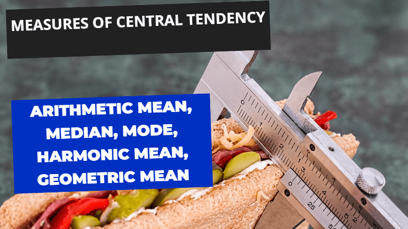
Measures of Central Tendency, Arithmetic Mean, Median, Mode, Harmonic, Geometric Mean