BCF Equation Solver – Solve Linear Equations Online | BCF Education. Solve systems of linear equations instantly with full step-by-step solutions. BCF Equation Solver supports 2 & 3 variable systems using Elimination, Matrix (Cramer’s Rule), and Gaussian methods. Free tool by BCF Education.
BCF Equation Solver – Solve Linear Equations Online | BCF Education
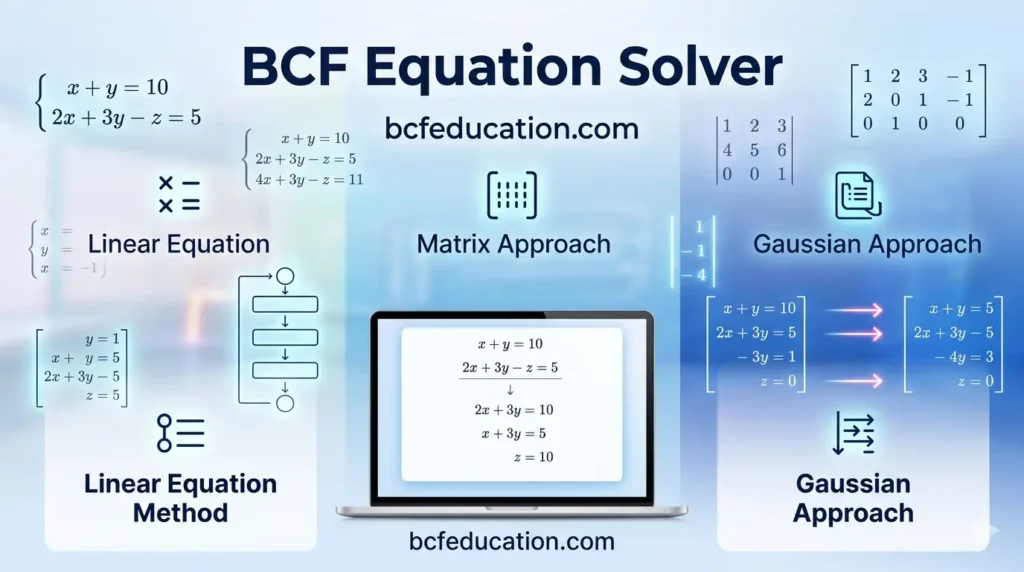
BCF Equation Solver
Instant Linear Systems Solver — bcfeducation.com
System of Linear Equations
2 VariablesTable of Contents
1 About the BCF Equation Solver
The BCF Equation Solver is a free, browser-based calculator designed for students, teachers, and professionals who need to solve systems of linear equations quickly and accurately. Unlike simple calculators that only show the answer, this tool provides complete step-by-step working for every calculation — making it an ideal learning companion as well as a productivity tool.
The solver supports systems with 2 variables (x, y) and 3 variables (x, y, z), and applies three internationally recognized mathematical methods: the Linear Elimination Method, the Matrix Method using Cramer’s Rule, and the Gaussian Elimination Method. All three methods are solved simultaneously from a single input, allowing users to compare approaches and deepen their understanding of linear algebra.
No sign-up, no download, and no payment required. The tool runs entirely in your browser and works on all devices — desktops, tablets, and smartphones.
1.2 Who Is This Tool For?
This tool is built for a wide range of users:
- University and college students studying Linear Algebra, Mathematics, Economics, Engineering, or Statistics.
- High school students learning simultaneous equations for the first time.
- Teachers and lecturers who want to generate step-by-step worked examples instantly.
- Researchers and professionals solving small linear systems as part of larger models.
- Anyone who needs a quick, reliable, and transparent equation solver online.
1.3 Key Features of the Tool
- Supports 2-variable and 3-variable systems of linear equations.
- Three complete solution methods with full step-by-step working shown.
- Add and delete equations and variables dynamically.
- Detects special cases: No Solution (inconsistent) and Infinite Solutions (dependent systems).
- Live equation preview updates as you type.
- Load built-in example problems with one click.
- Fully responsive — works perfectly on mobile, tablet, and desktop.
- No internet connection required after page load; runs client-side.
- Completely free with no registration required.
2. Educational Content — The Three Solution Methods
This section provides detailed educational descriptions of each method used by the BCF Equation Solver. This content can be published directly on your page, used in FAQs, or adapted for blog posts.
Method 1: Linear Equations Method (Elimination & Substitution)
What is the Linear Equations Method?
The Linear Equations Method is the most fundamental approach to solving systems of equations. It is typically the first method taught in algebra courses and forms the conceptual foundation for more advanced techniques. The method involves two core strategies — Elimination and Substitution — used together to reduce the system to simpler equations, one variable at a time.
How Does It Work?
The process begins by selecting one variable to eliminate from the system. Both equations are scaled (multiplied by appropriate constants) so that the chosen variable has equal coefficients. The equations are then added or subtracted to cancel that variable out, producing a new equation with one fewer variable. This process is repeated until a single-variable equation remains, which is solved directly. The resulting value is then back-substituted into previous equations to find all remaining variables.
Step-by-Step Process (2 Variables)
- Write both equations clearly, labelling them E1 and E2.
- Multiply E1 and E2 by appropriate multipliers so the coefficients of x are equal.
- Subtract one equation from the other to eliminate x.
- Solve the resulting single-variable equation for y.
- Substitute the value of y back into E1 to solve for x.
- Verify both values in E1 and E2 to confirm correctness.
When to Use This Method
- When coefficients are simple integers that make scaling easy.
- When teaching the foundational concepts of equation solving.
- For 2-variable systems where other methods may feel over-complicated.
- When one variable has the same or easily matchable coefficient across equations.
Special Cases
If, after elimination, the resulting equation is 0 = 0, the system has infinitely many solutions (the equations describe the same line or plane). If the result is 0 = k where k ≠ 0, the system has no solution (the lines or planes are parallel and do not intersect).
Real-World Applications
- Finding break-even points in business (cost vs. revenue equations).
- Solving mixture problems in chemistry and pharmacy.
- Network flow analysis in engineering.
- Balancing supply and demand in economics.
Method 2: Matrix Method — Cramer’s Rule
What is the Matrix Method?
The Matrix Method, specifically Cramer’s Rule, is an elegant algebraic technique that uses determinants to solve systems of linear equations. Named after the Swiss mathematician Gabriel Cramer (1704–1752), this method expresses a system of equations in the compact form A·X = B, where A is the coefficient matrix, X is the vector of unknowns, and B is the constants vector. Each variable is then computed as a ratio of determinants.
The Mathematical Foundation
Given a system of n equations in n unknowns, Cramer’s Rule states that each variable xᵢ is equal to the determinant of a modified matrix Aᵢ divided by the determinant of the original coefficient matrix A. The modified matrix Aᵢ is formed by replacing the i-th column of A with the constants column B.
(where det(A) ≠ 0 for a unique solution to exist)
Step-by-Step Process
- Express the system in matrix form: [A]·[X] = [B].
- Form the coefficient matrix [A] and the constants column [B].
- Calculate the main determinant: det(A).
- If det(A) = 0, the method cannot be applied (singular matrix).
- For each variable, replace the corresponding column of A with B to form Aᵢ.
- Compute det(Aᵢ) for each modified matrix.
- Divide each det(Aᵢ) by det(A) to obtain each variable.
- Verify results by substituting back into original equations.
Determinant Formulas
For a 2×2 matrix: det(A) = ad − bc
For a 3×3 matrix: Cofactor expansion along Row 1:
det(A) = a₁₁(a₂₂a₃₃ − a₂₃a₃₂) − a₁₂(a₂₁a₃₃ − a₂₃a₃₁) + a₁₃(a₂₁a₃₂ − a₂₂a₃₁)
Advantages of Cramer’s Rule
- Provides an explicit, direct formula for each variable — no iterative steps needed.
- Elegant and compact — ideal for theoretical proofs and symbolic computation.
- Easy to apply for 2×2 and 3×3 systems by hand.
- The determinant itself reveals important properties: if det(A) = 0, the system is singular.
Limitations
- Computationally expensive for large systems (not practical beyond 4×4 by hand).
- Cannot be applied if det(A) = 0.
- Does not naturally generalize to over-determined systems (more equations than unknowns).
Historical Note
Gabriel Cramer published this rule in 1750 in his “Introduction to the Analysis of Algebraic Curves.” Today it is a standard topic in linear algebra courses worldwide and is fundamental to understanding how determinants encode geometric information about linear systems.
Method 3: Gaussian Elimination Method
What is Gaussian Elimination?
Gaussian Elimination is one of the most important and widely used algorithms in numerical linear algebra. Named after the legendary German mathematician Carl Friedrich Gauss (1777–1855), it is the foundation of how computers solve large systems of linear equations. The method transforms the augmented matrix of a system into a simpler upper triangular (or row echelon) form, from which solutions are obtained by back-substitution.
The Augmented Matrix
The first step is to combine the coefficient matrix A and constants vector B into a single augmented matrix [A|B]. Each row of this matrix represents one equation, and each column (except the last) represents one variable. All operations are performed directly on rows of this matrix, making the process highly systematic and suitable for computer implementation.
| [ a₁₁ a₁₂ a₁₃ | b₁ ] [ a₂₁ a₂₂ a₂₃ | b₂ ] → Row Echelon Form → Back-Substitution [ a₃₁ a₃₂ a₃₃ | b₃ ] |
Elementary Row Operations
Gaussian Elimination uses three types of elementary row operations, all of which produce an equivalent system (same solution set):
- Row Swap: Exchange the positions of two rows (e.g., R₁ ↔ R₂).
- Row Scaling: Multiply all elements of a row by a non-zero constant.
- Row Addition: Add a multiple of one row to another row (Rᵢ = Rᵢ − mᵢⱼ × Rⱼ).
Step-by-Step Process
- Write the augmented matrix [A|B].
- Apply partial pivoting: move the row with the largest absolute pivot to the top (reduces rounding errors).
- For each pivot column, compute the elimination factor: mᵢⱼ = Aᵢⱼ / Aⱼⱼ.
- Subtract (mᵢⱼ × pivot row) from each row below to create zeros under the pivot.
- Repeat for each subsequent pivot position until upper triangular form is reached.
- Read the last equation (one variable), solve directly.
- Back-substitute upward, substituting known values to find remaining unknowns.
- Verify all solutions in the original equations.
Partial Pivoting
Partial pivoting is a crucial enhancement where rows are reordered so that the largest absolute value in a column is used as the pivot element. This prevents division by very small numbers, which would amplify rounding errors — especially important in computer-based computation. The BCF Equation Solver implements partial pivoting automatically.
Special Cases Detected
- No Solution: If a row of the form [0 0 … 0 | k] with k ≠ 0 appears, the system is inconsistent.
- Infinite Solutions: If a row of all zeros [0 0 … 0 | 0] appears, the system is dependent.
- Unique Solution: If the matrix reduces cleanly to upper triangular form without any of the above, a unique solution exists.
Why Gaussian Elimination Matters
- It is the basis for LU decomposition, used in engineering and scientific computing.
- It generalizes to any size system (n × n or even over/under-determined systems).
- It handles all three solution types naturally: unique, none, or infinite.
- Computational complexity is O(n³), making it efficient for moderate-size systems.
- Used in finite element analysis, computer graphics, economics modelling, and machine learning.
Historical Note
Although named after Gauss, this algorithm was known in China as early as 179 AD in the mathematical text “Sea Island Mathematical Manual.” It was independently developed in Europe in the 18th century. Today it is the canonical method for solving linear systems in computational mathematics.
5. Frequently Asked Questions (FAQ) — SEO Content
FAQs are highly valuable for SEO as they target question-based searches and may appear as Google featured snippets. Include these on your tool page in an accordion or expandable FAQ section.
Q: What is a system of linear equations?
A system of linear equations is a collection of two or more equations, each involving the same set of variables, all raised to the first power (linear). The goal is to find values of those variables that satisfy all equations simultaneously. For example, “2x + 3y = 8 and 5x − y = 2” is a 2-variable linear system.
Q: What does ‘step-by-step solution’ mean?
The BCF Equation Solver doesn’t just give the answer — it shows every mathematical operation performed at each stage. For each method, you see the multipliers used, the row operations applied, the intermediate equations formed, and the final back-substitution. This makes it ideal for checking homework, studying for exams, or understanding the method itself.
Q: What is the difference between the three methods?
All three methods solve the same problem but in different ways. The Elimination Method is the most intuitive and is taught first in schools. Cramer’s Rule uses determinants and gives a direct formula for each variable. Gaussian Elimination is the most systematic and powerful, transforming the system into a matrix and using row operations — it’s the basis for how computers solve equations.
Q: What if the system has no solution?
If the equations are contradictory (e.g., they represent parallel lines or planes that never intersect), the system is inconsistent and has no solution. The BCF Equation Solver detects this automatically and displays a ‘No Solution’ message with an explanation.
Q: What does ‘infinite solutions’ mean?
Infinite solutions occur when two or more equations in the system are actually the same equation written differently (dependent equations). Geometrically, the equations represent the same line or plane, so every point on that line/plane is a solution. The solver detects and reports this case.
Q: Can I use this tool for homework and exams?
The BCF Equation Solver is designed for learning and verification. Use it to check your own working, understand where you went wrong, or study a new method. The step-by-step solutions help you learn — not just get an answer.
Q: Is this tool free to use?
Yes. The BCF Equation Solver is completely free, requires no account or registration, and runs entirely in your browser. It is a service provided by BCF Education to support students, teachers, and learners worldwide.
Q: What is Cramer’s Rule?
Cramer’s Rule is a method for solving systems of linear equations using determinants. Each variable is computed as the ratio of two determinants: the numerator is the determinant of the coefficient matrix with the constants column substituted in, and the denominator is the determinant of the original coefficient matrix. It is applicable only when the main determinant is non-zero.
Q: What is Gaussian Elimination?
Gaussian Elimination is an algorithm that transforms the augmented matrix of a linear system into row echelon form (upper triangular matrix) using elementary row operations. Once in this form, the solution is found by back-substitution — solving the last equation first, then working upward.
Q: Why does BCF Education provide this tool for free?
BCF Education is committed to making quality educational resources accessible to all. This tool is part of our growing library of free online math and statistics tools designed to support learners at every level. Visit bcfeducation.com to explore more tools and resources.
