In this post, we are going to discuss, Statistics I HSSC I FBISE Solved Paper 2023, MCQS, Short Questions, Extensive Questions. Dive into the world of statistics with our comprehensive solutions to the Statistics I paper, covering key topics such as Introduction to Statistics, Measures of Central Tendency and Dispersion, Index Numbers, Correlation & Regression, and Time Series Analysis. Perfect for students and professionals alike, our detailed explanations will help you master these fundamental concepts. Explore more resources on statistical, economical, accounting, and finance topics at bcfeducation.com.
Other Solved Papers of Statistics I are available here.
Solved by Iftikhar Ali M.Sc. Economics, MCOM Finance Lecturer Statistics, Economics, Finance & Accounting
Table of Contents
Statistics I HSSC I FBISE Solved Paper 2023, MCQS, Short Questions, Extensive Questions
MCQS
Fill the relevant bubble against each question according to curriculum:
| 1 | The branch of statistics that is concerned with procedures for obtaining valid conditions is called: | ||
| A) | Descriptive Statistics | B) | Inferential Statistics |
| C) | Theoretical Statistics | D) | Applied Statistics |
| 2 | Issuing a National identity card is an example of: | ||
| A) | Census | B) | Registration |
| C) | Sampling | D) | Investigation through enumerators |
| 3 | The process of systematic arrangement of data into rows and columns is called: | ||
| A) | Classification | B) | Tabulation |
| C) | Frequency Distribution | D) | Array |
| 4 | An Ogive is also called: | ||
| A) | Frequency Polygon | B) | Frequency Curve |
| C) | Histogram | D) | Cumulative Frequency Polygon |
| 5 | The modal letter(s) of the word :STATISTICS” is/are: | ||
| A) | S | B) | T |
| C) | S,T | D) | I,T |
| 6 | If X̅ =10 and Y = 2X + 5, then Y̅ = __________: | ||
| A) | 10 | B) | 15 |
| C) | 20 | D) | 25 |
| 7 | The sum of squared deviations from mean is always: | ||
| A) | Negative | B) | Maximum |
| C) | Minimum | D) | Zero |
| 8 | Geometric mean of 2, 4, 6, 8, 64 is: | ||
| A) | 7 | B) | 7.55 |
| C) | 16.8 | D) | 8.5 |
| 9 | For normal distribution, approximately 68% of the values are included by an interval: | ||
| A) | X̅±S | B) | X̅±2S |
| C) | X̅±3S | D) | X̅±4S |
| 10 | If Var(X) = 2, then Var(3X +4) = _______: | ||
| A) | 10 | B) | 15 |
| C) | 18 | D) | 20 |
| 11 | The reversal test is satisfied by: | ||
| A) | Laspeyre’s Index | B) | Paasche’s Index |
| C) | Fisher’s Index | D) | Un-weighted Index Number |
| 12 | The index number is given by (∑pnqn/∑poqn)x100 is called: | ||
| A) | The Laspeyre’s index | B) | The Paasche’s index |
| C) | The value index | D) | Wholesale price index |
| 13 | The price relative is the percentage ratio of current year price and: | ||
| A) | Current year quantity | B) | Base year quantity |
| C) | Current year price | D) | Base year price |
| 14 | In method of least square, the sum of errors will be: | ||
| A) | Less than zero | B) | Greater than zero |
| C) | Zero | D) | Not equal to zero |
| 15 | The regression line always passing through: | ||
| A) | (a, Y̅) | B) | (b, Y̅) |
| C) | (a,b) | D) | (X̅,Y̅) |
| 16 | When two variables move in same direction, the correlation will be: | ||
| A) | Positive | B) | Negative |
| C) | Zero | D) | Neutral |
| 17 | A decline in death rate due to advancement of Science is an example of: | ||
| A) | Seasonal Variation | B) | Secular Variation |
| C) | Cyclical Variation | D) | Random Variation |
Total Marks Sections B and C: 68
Note: Answer any fourteen parts from section “B” and any two questions from Section “C”. Write your answers neatly and legibly. Statistical table will be provided on demand.
Section B- (Marks 42)
Short Questions
(i) Distinguish between primary and secondary data.
Answer
First hand, newly collected, ungrouped data is called primary data or data which is not collected by someone previously is called primary data.
Second hand, previously collected, grouped data is called secondary data or data which is collected by someone previously is called secondary data.
(ii) Differentiate between discrete variable and continuous variable.
Answer:
Discrete Variable
Discrete variable is a variable in which a data has some specific value within a given range or we can say that discrete variable has variable that is countable. For example, number of persons, number of cars, number of students etc.
Continuous Variable
Continuous variable is a variable in which a data has any value within a given range or we can say that continuous variable has variable that is measurable. For example, height of students, speed of car, length of wood etc.
(iii) Make class boundaries and find missing frequencies of the following frequency distributions.
| Classes | Frequency | Cumulative Frequency |
| 0.7312—0.7313 | 5 | 5 |
| 0.7314—0.7315 | 7 | ? |
| 0.7316—0.7317 | ? | 22 |
| 0.7318—0.7319 | 8 | ? |
| 0.7320—0.7321 | ? | 35 |
Solution:
| Classes | Frequency | Cumulative Frequency |
| 0.7312—0.7313 | 5 | 5 |
| 0.7314—0.7315 | 7 | 5+7=12 |
| 0.7316—0.7317 | 22-12=10 | 22 |
| 0.7318—0.7319 | 8 | 22+8=30 |
| 0.7320—0.7321 | 35-30=5 | 35 |
(iv) Calculate Arithmetic mean from the following deviations.
| D=X-10 | -5 | -3 | 0 | 3 | 6 | 8 | 10 | 13 |
Solution:
| D=X-10 | -5 | -3 | 0 | 3 | 6 | 8 | 10 | 13 | ∑D=32 |
![\[ \mathbf{A.M\ \ }\overline{\mathbf{X}}\mathbf{= A +}\frac{\mathbf{\sum D}}{\mathbf{n\ }}\ \]](https://bcfeducation.com/wp-content/ql-cache/quicklatex.com-bf0d57be9ba29a3e1997be457c42ede3_l3.png "Rendered by QuickLaTeX.com")
![\[ \mathbf{A.M\ \ }\overline{\mathbf{X}}\mathbf{= 10 +}\frac{\mathbf{32}}{\mathbf{8}}\ \]](https://bcfeducation.com/wp-content/ql-cache/quicklatex.com-bf4161f60ea3b5a0a13aeea3eaf23471_l3.png "Rendered by QuickLaTeX.com")
![\[ \mathbf{A.M = 14}\ \]](https://bcfeducation.com/wp-content/ql-cache/quicklatex.com-57fed6a9c6d89c1c294f2676c03bad43_l3.png "Rendered by QuickLaTeX.com")
(v) Calculate Geometric Mean and Harmonic Mean for five values of X for the following reciprocal values:
| 1/X | 0.2 | 0.1 | 0.05 | 0.04 | 0.025 |
Solution:
| 1/X | X=1/1/x |
| 0.2 | 5 |
| 0.1 | 10 |
| 0.05 | 20 |
| 0.04 | 25 |
| 0.025 | 40 |
| ∑(1/X)=0.415 |
![\[ \mathbf{Harmonic\ Mean =}\frac{\mathbf{n}}{\mathbf{\sum}\left( \frac{\mathbf{1}}{\mathbf{x}} \right)}\ \]](https://bcfeducation.com/wp-content/ql-cache/quicklatex.com-37d7466142ee12cfa2aadaa49193c7a4_l3.png "Rendered by QuickLaTeX.com")
![\[ \mathbf{Harmonic\ Mean =}\frac{\mathbf{5}}{\mathbf{0.415}}\ \]](https://bcfeducation.com/wp-content/ql-cache/quicklatex.com-78ef0fca8066e80558c3f204f135baa4_l3.png "Rendered by QuickLaTeX.com")
![\[ \mathbf{Harmonic\ Mean = 12}\ \]](https://bcfeducation.com/wp-content/ql-cache/quicklatex.com-9f18526be6390ae03541c8d3d99af134_l3.png "Rendered by QuickLaTeX.com")
![\[ \mathbf{G.M =}\mathbf{(5 \times 10 \times 20 \times 25 \times 40)}^{\frac{\mathbf{1}}{\mathbf{5}}}\ \]](https://bcfeducation.com/wp-content/ql-cache/quicklatex.com-d8c1773631118a299ba23e13491b2e86_l3.png "Rendered by QuickLaTeX.com")
![\[ \mathbf{G.M = 15.84}\ \]](https://bcfeducation.com/wp-content/ql-cache/quicklatex.com-ccf705b0dcdf28ffb4dd5c18ea56b131_l3.png "Rendered by QuickLaTeX.com")
(vi) Calculate combined Arithmetic mean for the following two groups.
| Boys | Girls | |
| Number of Persons | 20 | 30 |
| Mean Weight (kg) | 62.5 | 53.4 |
Solution:
![\[ \overline{\mathbf{X}}\mathbf{c =}\frac{\overline{\mathbf{X}}\mathbf{1}\mathbf{n}\mathbf{1 +}\overline{\mathbf{X}}\mathbf{2}\mathbf{n}\mathbf{2}}{\mathbf{n}\mathbf{1 + n}\mathbf{2}}\ \]](https://bcfeducation.com/wp-content/ql-cache/quicklatex.com-9643697d574a761e8ce51b399c190c7b_l3.png "Rendered by QuickLaTeX.com")
![\[ \overline{\mathbf{X}}\mathbf{c =}\frac{\left( \mathbf{62.5 \times 20} \right)\mathbf{+ (53.4 \times 30)}}{\mathbf{20 + 30}}\ \]](https://bcfeducation.com/wp-content/ql-cache/quicklatex.com-9d5f54455f985d8e79c3b7901842a46c_l3.png "Rendered by QuickLaTeX.com")
![\[ \overline{\mathbf{X}}\mathbf{c =}\frac{\mathbf{1250 + 1602}}{\mathbf{50}}\ \]](https://bcfeducation.com/wp-content/ql-cache/quicklatex.com-362425d31ae898c008ec84ce6b3906ac_l3.png "Rendered by QuickLaTeX.com")
![\[ \overline{\mathbf{X}}\mathbf{c = 57.04}\ \]](https://bcfeducation.com/wp-content/ql-cache/quicklatex.com-c4717e787c27244bf4af51e00ffff560_l3.png "Rendered by QuickLaTeX.com")
(vii) What is meant by range and semi-interquartile range?
Answer: Range and semi-interquartile range both are absolute measures of dispersion. Range calculates the dispersion of class marks and semi interquartile deviation or quartile deviation calculates the dispersion of quartiles. Formulas are given below:
![\[ Range\ = \ Xm\ -\ Xo\ \]](https://bcfeducation.com/wp-content/ql-cache/quicklatex.com-e2558ea62a1a988a5258ccb078c42618_l3.png "Rendered by QuickLaTeX.com")
![\[ Quartile\ Deviation\ or\ S.I.Q.R = \ \frac{Q3 - Q1}{2}\ \]](https://bcfeducation.com/wp-content/ql-cache/quicklatex.com-cf6017b75fad3f44a798864e856c0677_l3.png "Rendered by QuickLaTeX.com")
(viii) If lower quartile (Q1) = 40, upper quartile (Q3) = 90 and Median = 60, Compute Quartile Coefficient of Skewness.
Solution:
![\[ \mathbf{Quartile\ Coefficient\ of\ Skewness =}\frac{\mathbf{Q3 + Q1 - 2Median}}{\mathbf{Q3 - Q1}}\ \]](https://bcfeducation.com/wp-content/ql-cache/quicklatex.com-f12dba63679b0d80f2c512455f3c9e93_l3.png "Rendered by QuickLaTeX.com")
![\[ \mathbf{Quartile\ Coefficient\ of\ Skewness =}\frac{\mathbf{90}\mathbf{+}\mathbf{40}\mathbf{- 2}\mathbf{(60)}}{\mathbf{90 - 40}}\ \]](https://bcfeducation.com/wp-content/ql-cache/quicklatex.com-85503d14891c57878bbf32f867aac563_l3.png "Rendered by QuickLaTeX.com")
![\[ \mathbf{Quartile\ Coefficient\ of\ Skewness =}\frac{\mathbf{10}}{\mathbf{50}}\mathbf{= 0.2}\ \]](https://bcfeducation.com/wp-content/ql-cache/quicklatex.com-be2f09270730a7cec1561b3408ff9c9a_l3.png "Rendered by QuickLaTeX.com")
(ix) Given n =5, ∑x=180, ∑x²=6660. Compute variance, Standard deviation and coefficient of variation.
Solution:
![\[ \mathbf{Variance\ }\mathbf{S}^{\mathbf{2}}\mathbf{=}\frac{\mathbf{\sum}\mathbf{x}^{\mathbf{2}}}{\mathbf{n}}\mathbf{-}\left( \frac{\mathbf{\sum x}}{\mathbf{n}} \right)^{\mathbf{2}}\ \]](https://bcfeducation.com/wp-content/ql-cache/quicklatex.com-efbf055c00f5594e2250bf3f52a13840_l3.png "Rendered by QuickLaTeX.com")
![\[ \mathbf{Variance\ }\mathbf{S}^{\mathbf{2}}\mathbf{=}\frac{\mathbf{6660}}{\mathbf{5}}\mathbf{-}\left( \frac{\mathbf{180}}{\mathbf{5}} \right)^{\mathbf{2}}\ \]](https://bcfeducation.com/wp-content/ql-cache/quicklatex.com-78fe0783bffdc6ff3df4fc1a0c6d877d_l3.png "Rendered by QuickLaTeX.com")
![\[ \mathbf{Variance\ }\mathbf{S}^{\mathbf{2}}\mathbf{= 1332 - 1296}\ \]](https://bcfeducation.com/wp-content/ql-cache/quicklatex.com-6cd96d54a94177a2a3fe8b940c7043eb_l3.png "Rendered by QuickLaTeX.com")
![\[ \mathbf{Variance\ }\mathbf{S}^{\mathbf{2}}\mathbf{= 36}\ \]](https://bcfeducation.com/wp-content/ql-cache/quicklatex.com-4a53086afa0dab92471b58c66025af61_l3.png "Rendered by QuickLaTeX.com")
![\[ \mathbf{Standard\ Deviation\ S =}\sqrt{\frac{\mathbf{\sum}\mathbf{x}^{\mathbf{2}}}{\mathbf{n}}\mathbf{-}\left( \frac{\mathbf{\sum x}}{\mathbf{n}} \right)^{\mathbf{2}}\mathbf{\ }}\ \]](https://bcfeducation.com/wp-content/ql-cache/quicklatex.com-c63918af64fdae140755b0777325eaba_l3.png "Rendered by QuickLaTeX.com")
![\[ \mathbf{Standard\ Deviation\ S =}\sqrt{\mathbf{36}\mathbf{\ }}\ \]](https://bcfeducation.com/wp-content/ql-cache/quicklatex.com-2c7faa9d7b4c97950273c665f5adb630_l3.png "Rendered by QuickLaTeX.com")
![\[ \mathbf{Standard\ Deviation\ S = 6}\ \]](https://bcfeducation.com/wp-content/ql-cache/quicklatex.com-b32b3296bb8278155bfa30bb6f48b235_l3.png "Rendered by QuickLaTeX.com")
![\[ \mathbf{Mean =}\frac{\mathbf{\sum x}}{\mathbf{n}}\mathbf{=}\frac{\mathbf{180}}{\mathbf{5}}\mathbf{= 36}\ \]](https://bcfeducation.com/wp-content/ql-cache/quicklatex.com-997f25e8771860a0b07183e5b43db399_l3.png "Rendered by QuickLaTeX.com")
![\[ \mathbf{C.V =}\frac{\mathbf{S.D}}{\mathbf{Mean}}\mathbf{\times}\mathbf{100}\ \]](https://bcfeducation.com/wp-content/ql-cache/quicklatex.com-4a21057805bd7dbbf5a8dc5a766f97cd_l3.png "Rendered by QuickLaTeX.com")
![\[ \mathbf{C.V =}\frac{\mathbf{6}}{\mathbf{36}}\mathbf{\times}\mathbf{100}\ \]](https://bcfeducation.com/wp-content/ql-cache/quicklatex.com-8c1e96f076300fc0e2a58565eedc531e_l3.png "Rendered by QuickLaTeX.com")
![\[ \mathbf{C.V = 16.67}\ \]](https://bcfeducation.com/wp-content/ql-cache/quicklatex.com-4a4744378912efd97665b4e4864410fe_l3.png "Rendered by QuickLaTeX.com")
(x) Differentiate between un-weighted and weighted index number.
Answer:
Un-weighted Index Number
Un-weighted index number is a measure of composite index number. In un-weighted index number, weights or quantities are not given. Unweighted index numbers are calculated through following methods:
- Aggregative Index
- Average of Relative Method
Weighted Index
Weighted index is also a measure of composite index numbers in which weights or quantities are given. Weighted index can be calculated through number of methods given below:
- Laspeyre’s Method
- Paasche’s Method
- Fisher’s Ideal Index Method
- Marshal Edgesworth Method
- Walsh Method
(xi) Compute index number taking 2010 as base:
| Year | 2010 | 2011 | 2012 | 2013 | 2014 | 2015 |
| Price | 10 | 14 | 15 | 20 | 25 | 33 |
Solution:
| Year | Price | Index Number taking 2010 as base |
| 2010 | 10 | |
| 2011 | 14 | |
| 2012 | 15 | |
| 2013 | 20 | |
| 2014 | 25 | |
| 2015 | 33 | |
![\[ \left( \frac{\mathbf{10}}{\mathbf{10}} \right)\mathbf{100\ = \ 100}\ \]](https://bcfeducation.com/wp-content/ql-cache/quicklatex.com-05f38fd69ecea7ce9539da3dcbf1e204_l3.png "Rendered by QuickLaTeX.com")
![\[ \left( \frac{\mathbf{14}}{\mathbf{10}} \right)\mathbf{100\ = \ 140}\ \]](https://bcfeducation.com/wp-content/ql-cache/quicklatex.com-ca0474a9cc3681217749f104700945f3_l3.png "Rendered by QuickLaTeX.com")
![\[ \left( \frac{\mathbf{15}}{\mathbf{10}} \right)\mathbf{100\ = \ 150}\ \]](https://bcfeducation.com/wp-content/ql-cache/quicklatex.com-99b6c8444fa2ecebce6a9ae63cc633d9_l3.png "Rendered by QuickLaTeX.com")
![\[ \left( \frac{\mathbf{20}}{\mathbf{10}} \right)\mathbf{100\ = \ 200}\ \]](https://bcfeducation.com/wp-content/ql-cache/quicklatex.com-a037612d3c666ab4624652d9ccd1b127_l3.png "Rendered by QuickLaTeX.com")
![\[ \left( \frac{\mathbf{25}}{\mathbf{10}} \right)\mathbf{100\ = \ 250}\ \]](https://bcfeducation.com/wp-content/ql-cache/quicklatex.com-784620c4b2d8ab5fc10e86640836b5bf_l3.png "Rendered by QuickLaTeX.com")
![\[ \left( \frac{\mathbf{33}}{\mathbf{10}} \right)\mathbf{100\ = \ 330}\ \]](https://bcfeducation.com/wp-content/ql-cache/quicklatex.com-c5b3ec1a033156027a9f1b644ebb4c61_l3.png "Rendered by QuickLaTeX.com")
(xii) If Laspeyre’s index number is 150 and Fisher’s index is 147, calculate the Paasche’s index number.
Solution:
![\[ \mathbf{Fishe}\mathbf{r}^{\mathbf{'}}\mathbf{s\ Index =}\sqrt{\mathbf{L \times P}}\ \]](https://bcfeducation.com/wp-content/ql-cache/quicklatex.com-a03e7c981018e145b2593f56ad530fbb_l3.png "Rendered by QuickLaTeX.com")
![\[ \mathbf{147 =}\sqrt{\mathbf{150 \times P}}\ \]](https://bcfeducation.com/wp-content/ql-cache/quicklatex.com-5140569efdf6bb0017eb517019f3b367_l3.png "Rendered by QuickLaTeX.com")
Taking square root on both sides:
![\[ \mathbf{(147)}^{\mathbf{2}}\mathbf{=}\left( \sqrt{\mathbf{150}} \right)^{\mathbf{2}}\mathbf{\times}\left( \sqrt{\mathbf{P}} \right)^{\mathbf{2}}\ \]](https://bcfeducation.com/wp-content/ql-cache/quicklatex.com-de8713a73e9c4cc94155f25a432f3fb9_l3.png "Rendered by QuickLaTeX.com")
![\[ \mathbf{21609 = 150 \times P}\ \]](https://bcfeducation.com/wp-content/ql-cache/quicklatex.com-771cbad402a317fdd7cee4099b3705cd_l3.png "Rendered by QuickLaTeX.com")
![\[ \mathbf{P =}\frac{\mathbf{21609}}{\mathbf{150}}\mathbf{= 144.06}\ \]](https://bcfeducation.com/wp-content/ql-cache/quicklatex.com-73d3d460860dae6d5ecc94ba24bbbe7b_l3.png "Rendered by QuickLaTeX.com")
![\[ \mathbf{Paasche}\mathbf{s}^{\mathbf{'}}\mathbf{s\ Index = 144.06}\ \]](https://bcfeducation.com/wp-content/ql-cache/quicklatex.com-c2f06009a6084a41a5599821c091f66d_l3.png "Rendered by QuickLaTeX.com")
(xiii) Compute two regression coefficients byx and bxy of following data: n=10, ∑Dx=12, ∑Dy=-5, ∑DxDy=390,∑Dx²=2830, ∑Dy²=91
Solution:
Regression Coefficient y on x:
![\[ \mathbf{b}_{\mathbf{yx}}\mathbf{=}\frac{\mathbf{\sum DxDy -}\frac{\mathbf{(\sum Dx)(\sum Dy)}}{\mathbf{n}}}{\mathbf{\sum}\mathbf{Dx}^{\mathbf{2}}\mathbf{-}\frac{\left( \mathbf{\sum Dx} \right)^{\mathbf{2}}}{\mathbf{n}}}\ \]](https://bcfeducation.com/wp-content/ql-cache/quicklatex.com-ac63e1d793a7e8f10eb164fc4defb9b5_l3.png "Rendered by QuickLaTeX.com")
![\[ \mathbf{b}_{\mathbf{yx}}\mathbf{=}\frac{\mathbf{390}\mathbf{-}\frac{\mathbf{(}\mathbf{12}\mathbf{)(}\mathbf{- 5}\mathbf{)}}{\mathbf{10}}}{\mathbf{2830}\mathbf{-}\frac{\left( \mathbf{12} \right)^{\mathbf{2}}}{\mathbf{10}}}\ \]](https://bcfeducation.com/wp-content/ql-cache/quicklatex.com-3e41f4bbc5340bd3e0187646aac5b7b8_l3.png "Rendered by QuickLaTeX.com")
![\[ \mathbf{b}_{\mathbf{yx}}\mathbf{=}\frac{\mathbf{39}\mathbf{6}}{\mathbf{28}\mathbf{15.6}}\ \]](https://bcfeducation.com/wp-content/ql-cache/quicklatex.com-c53812a269eef550d9bd35130aac9270_l3.png "Rendered by QuickLaTeX.com")
![\[ \mathbf{b}_{\mathbf{yx}}\mathbf{=}\mathbf{0.140}\ \]](https://bcfeducation.com/wp-content/ql-cache/quicklatex.com-f2bdf13620b1ff2cb6baf31a2426fddc_l3.png "Rendered by QuickLaTeX.com")
Regression Coefficient x on y:
![\[ \mathbf{b}_{\mathbf{yx}}\mathbf{=}\frac{\mathbf{\sum DxDy -}\frac{\mathbf{(\sum Dx)(\sum Dy)}}{\mathbf{n}}}{\mathbf{\sum}{\mathbf{D}\mathbf{y}}^{\mathbf{2}}\mathbf{-}\frac{\left( \mathbf{\sum D}\mathbf{y} \right)^{\mathbf{2}}}{\mathbf{n}}}\ \]](https://bcfeducation.com/wp-content/ql-cache/quicklatex.com-c2d91f1d68e77aa712e2285529e837ed_l3.png "Rendered by QuickLaTeX.com")
![\[ \mathbf{b}_{\mathbf{yx}}\mathbf{=}\frac{\mathbf{390 -}\frac{\mathbf{(}\mathbf{12}\mathbf{)(}\mathbf{- 5}\mathbf{)}}{\mathbf{10}}}{\mathbf{91}\mathbf{-}\frac{\left( \mathbf{- 5} \right)^{\mathbf{2}}}{\mathbf{10}}}\ \]](https://bcfeducation.com/wp-content/ql-cache/quicklatex.com-4e08d148e027ee90d524d500b2382e87_l3.png "Rendered by QuickLaTeX.com")
![\[ \mathbf{b}_{\mathbf{yx}}\mathbf{=}\frac{\mathbf{396}}{\mathbf{88.5}}\ \]](https://bcfeducation.com/wp-content/ql-cache/quicklatex.com-4c401ac2f9719665c84427440aecb863_l3.png "Rendered by QuickLaTeX.com")
![\[ \mathbf{b}_{\mathbf{yx}}\mathbf{=}\mathbf{4.47}\ \]](https://bcfeducation.com/wp-content/ql-cache/quicklatex.com-abe4e00ccafc49404f9e38000179f2b0_l3.png "Rendered by QuickLaTeX.com")
(iv) The two regression lines are Ŷ=25+0.83x and X̂=40+0.97y are given, identify the two regression coefficients and compute the correlation coefficient (r).
Solution:
Regression Coefficient Y on X
![\[ \mathbf{b}_{\mathbf{yx}}\mathbf{= 0.83}\ \]](https://bcfeducation.com/wp-content/ql-cache/quicklatex.com-74bcd93bf5b1fe4c5ee1d22bf00d413f_l3.png "Rendered by QuickLaTeX.com")
Regression Coefficient X on Y
![\[ \mathbf{b}_{\mathbf{xy}}\mathbf{= 0.97}\ \]](https://bcfeducation.com/wp-content/ql-cache/quicklatex.com-d2fc9db75d4a30e35a04ec29f701df7f_l3.png "Rendered by QuickLaTeX.com")
Correlation Coefficient
![\[ \mathbf{r}{\mathbf{xy}}\mathbf{=}\sqrt{\left( \mathbf{b}{\mathbf{yx}} \right)\mathbf{(}\mathbf{b}_{\mathbf{xy}}\mathbf{)}}\ \]](https://bcfeducation.com/wp-content/ql-cache/quicklatex.com-7a000b089359efd844cb71ade2753e68_l3.png "Rendered by QuickLaTeX.com")
![\[ \mathbf{r}_{\mathbf{xy}}\mathbf{=}\sqrt{\left( \mathbf{0.83} \right)\mathbf{(0.97)}}\ \]](https://bcfeducation.com/wp-content/ql-cache/quicklatex.com-a062c06d74c588454c51f3e92d3b75ce_l3.png "Rendered by QuickLaTeX.com")
![\[ \mathbf{r}_{\mathbf{xy}}\mathbf{=}\sqrt{\mathbf{0.8051}}\ \]](https://bcfeducation.com/wp-content/ql-cache/quicklatex.com-9d9668def813347441668115a6713c88_l3.png "Rendered by QuickLaTeX.com")
![\[ \mathbf{r}_{\mathbf{xy}}\mathbf{= 0.8972}\ \]](https://bcfeducation.com/wp-content/ql-cache/quicklatex.com-4646b03b034fc0e644946675d51c64bf_l3.png "Rendered by QuickLaTeX.com")
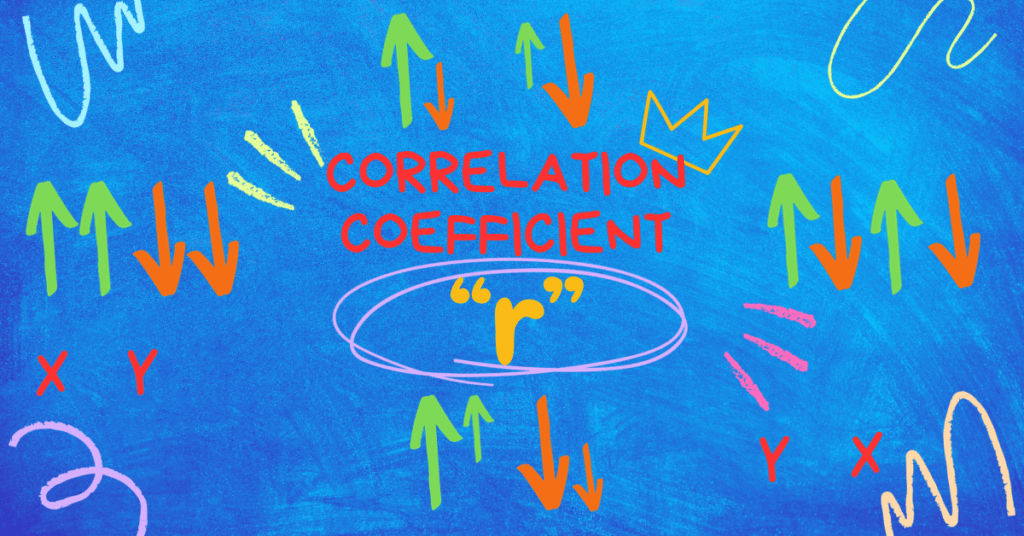
(xv) Write down the properties of correlation coefficient (r).
Answer:
1. Symmetric Property
Correlation between X variable and Y variable and Y Variable and X variable have same meaning or:
![\[ \mathbf{r}{\mathbf{xy}}\mathbf{=}\mathbf{r}{\mathbf{yx}}\ \]](https://bcfeducation.com/wp-content/ql-cache/quicklatex.com-bb660589f7e9cc61c8eafd6801f8d79b_l3.png "Rendered by QuickLaTeX.com")
2. Free from unit of measurement
Correlation coefficient is free from unit of measurement means if data is given in kilograms or length, the answer will not be in kilograms or length.
3. Independent to Origin and Scale
Correlation Coefficient is independent to origin and scale means:
![\[ r_{xy} = r_{uv}\ where\ U = \ \frac{X \pm A}{h}\ and\ V = \frac{Y \pm B}{h}\ \]](https://bcfeducation.com/wp-content/ql-cache/quicklatex.com-dc276b7edd286cc707e2e3492f529289_l3.png "Rendered by QuickLaTeX.com")
4. Range of Correlation Coefficient
Correlation Coefficient always lies between -1 to +1 both inclusive.
5. Geometric Mean of Regression Coefficients
Correlation Coefficient is a geometric mean of two regression coefficients.
![\[ \mathbf{r}_{\mathbf{xy}}\mathbf{=}\sqrt{\mathbf{byx\ \times bxy}}\ \]](https://bcfeducation.com/wp-content/ql-cache/quicklatex.com-6d4b5ad78fa587b10a6798fab57b7545_l3.png "Rendered by QuickLaTeX.com")
6. Relation with Covariance
If X and Y are two independent variables then Cov(X, Y) = 0 but it does not mean that if Cov (X, Y) = 0 then X and Y are definitely independent.
(xvi) If rxy =0.60, U=(X – 50)/10, V = (Y – 60)/5, then what is the value of rxy and ruv?
Answer: It is the property of correlation coefficient that it is independent to origin and scale so rxy is equals to ruv and its value is 0.60.
(xvii) Describe seasonal variation with example in time series.
Answer: Seasonal variation is a variation of time series that occurs repeatedly when season changes. For example, in summer, the demand for cold drinks increases and when winter comes it reduces and this happens again and again.
(xviii) If the least square line fitted to the data for the years 1960-65 (both inclusive) with the origin at the middle of 1962 and 1963 is Ŷ = 75+0.85x, the unit of X is being half year, then find the trend values for 1960 to 1965.
Solution:
| Year | X | Trend Values Ŷ = 75+0.85x |
| 1960 | -2.5 | Ŷ = 75+0.85(-2.5)=72.875 |
| 1961 | -1.5 | Ŷ = 75+0.85(-1.5)=73.725 |
| 1962 | -0.5 | Ŷ = 75+0.85(-0.5)=74.575 |
| 1963 | +0.5 | Ŷ = 75+0.85(0.5)=75.425 |
| 1964 | +1.5 | Ŷ = 75+0.85(1.5)=76.275 |
| 1965 | +2.5 | Ŷ = 75+0.85(2.5)=77.125 |
(xix) Estimate the trend values by semi average method for 1970 to 1975.
| Year | Semi-Total | Semi-Average |
| 1970 | ||
| 1971 | 720 | 240 |
| 1972 | ||
| 1973 | ||
| 1974 | 990 | 330 |
| 1975 |
Solution:
| Year | Semi-Total | Semi-Average | Trend Values Y̑ |
| 1970 | 240 – 30 = 210 | ||
| 1971 | 720 | 240 | 240 |
| 1972 | 240 + 30 = 270 | ||
| 1973 | 270 + 30 = 300 | ||
| 1974 | 990 | 330 | 330 |
| 1975 | 330 + 30 = 360 |
Increase of trend in 3 years = 330 – 240 = 90
Increase of trend in one year = 90/3 = 30
Section C Marks 26
Note: Attempt any two questions. All questions carry equal marks.
Extensive Questions
Q.3 a. Find Arithmetic Mean, Median and Mode from the following data: (06)
Q.3 a. Find Arithmetic Mean, Median and Mode from the following data: (06)
| Classes | 10-14 | 15-19 | 20-24 | 25-29 | 30-34 | 35-39 |
| Frequency | 3 | 5 | 10 | 12 | 6 | 4 |
Solution:
| Classes | Frequency | Class Boundaries | X | fx | C.F |
| 10—14 | 3 | 9.5–14.5 | 12 | 36 | 3 |
| 15—19 | 5 | 14.5–19.5 | 17 | 85 | 8 |
| 20—24 | 10 | 19.5–24.5 | 22 | 220 | 18 |
| 25—29 | 12 | 24.5–29.5 | 27 | 324 | 30 |
| 30—34 | 6 | 29.5–34.5 | 32 | 192 | 36 |
| 35—39 | 4 | 34.5–39.5 | 37 | 148 | 40 |
| ∑f =n= 40 | ∑fx = 1005 |
![\[ \mathbf{Mean =}\frac{\mathbf{\sum fx}}{\mathbf{\sum f}}\ \]](https://bcfeducation.com/wp-content/ql-cache/quicklatex.com-7046f10d591112c845e8a48cf6ca0656_l3.png "Rendered by QuickLaTeX.com")
![\[ \mathbf{Mean =}\frac{\mathbf{1005}}{\mathbf{40}}\mathbf{= 25.125}\ \]](https://bcfeducation.com/wp-content/ql-cache/quicklatex.com-bcc4191e8b4fa4fa67c79866d859d0b8_l3.png "Rendered by QuickLaTeX.com")
![\[ \mathbf{Median = l +}\frac{\mathbf{h}}{\mathbf{f}}\mathbf{(}\frac{\mathbf{n}}{\mathbf{2}}\mathbf{- c)}\ \]](https://bcfeducation.com/wp-content/ql-cache/quicklatex.com-51cdddb17d71bd4f7d7cd347b3aac7d2_l3.png "Rendered by QuickLaTeX.com")
n/2=40/2=20 falls in c.f of 30 so l=24.5, h=5,f=12,n/2=20, c=18
![\[ \mathbf{Median = 24.5 +}\frac{\mathbf{5}}{\mathbf{12}}\mathbf{(20 - 18)}\ \]](https://bcfeducation.com/wp-content/ql-cache/quicklatex.com-3ce2c0433499405c77996dc6649ab63d_l3.png "Rendered by QuickLaTeX.com")
![\[ \mathbf{Median = 25.33}\ \]](https://bcfeducation.com/wp-content/ql-cache/quicklatex.com-4633a62fe81f7932af7e4cd3f6531384_l3.png "Rendered by QuickLaTeX.com")
![\[ \mathbf{Mode = l +}\frac{\mathbf{(fm - f}\mathbf{1)}}{\left( \mathbf{fm - f}\mathbf{1} \right)\mathbf{+ (fm - f}\mathbf{2)}}\mathbf{\times h}\ \]](https://bcfeducation.com/wp-content/ql-cache/quicklatex.com-8ddadcc8941465771d00e4e1a2846241_l3.png "Rendered by QuickLaTeX.com")
Maximum frequency is 12 so l = 24.5, fm =12, f1=10, f2=6 and h = 5
![\[ \mathbf{Mode = 24.5 +}\frac{\mathbf{12 - 10}}{\left( \mathbf{12 - 10} \right)\mathbf{+ (12 - 6)}}\mathbf{\times 5}\ \]](https://bcfeducation.com/wp-content/ql-cache/quicklatex.com-ad8093185a7670af26a47a035f6b18b5_l3.png "Rendered by QuickLaTeX.com")
![\[ \mathbf{Mode = 24.5 +}\frac{\mathbf{10}}{\mathbf{8}}\mathbf{= 25.75}\ \]](https://bcfeducation.com/wp-content/ql-cache/quicklatex.com-a5d48f6b8e369a3512f11821a611b51e_l3.png "Rendered by QuickLaTeX.com")
b. Calculate Coefficient of skewness by Karl Pearson’s Methods. (07)
b. Calculate Coefficient of skewness by Karl Pearson’s Methods. (07)
| Marks | 20—24 | 25—29 | 30—34 | 35—39 | 40—44 | 45—49 |
| Frequency | 1 | 4 | 8 | 11 | 15 | 6 |
Solution:
| Classes | Frequency | Class Boundaries | X | fx | fx² |
| 20—24 | 1 | 19.5–24.5 | 22 | 22 | 484 |
| 25—29 | 4 | 24.5–29.5 | 27 | 108 | 2916 |
| 30—34 | 8 | 29.5–34.5 | 32 | 256 | 8192 |
| 35—39 | 11 | 34.5–39.5 | 37 | 407 | 15059 |
| 40—44 | 15 | 39.5–44.5 | 42 | 630 | 26460 |
| 45—49 | 6 | 44.5–49.5 | 47 | 282 | 13254 |
| ∑f =n= 45 | ∑fx = 1705 | ∑fx² = 66365 |
![\[ \mathbf{Karl\ Person}\mathbf{s}^{\mathbf{'}}\mathbf{s\ C.Skewness =}\frac{\mathbf{Mean - Mode}}{\mathbf{S.D}}\ \]](https://bcfeducation.com/wp-content/ql-cache/quicklatex.com-bfa3181a393af4963b892d6dcf24f774_l3.png "Rendered by QuickLaTeX.com")
![\[ \mathbf{Mean =}\frac{\mathbf{1705}}{\mathbf{45}}\mathbf{= 37.88}\ \]](https://bcfeducation.com/wp-content/ql-cache/quicklatex.com-bb2755e111497c125cc5cfb4ffd38c5f_l3.png "Rendered by QuickLaTeX.com")
Maximum frequency is 15 so l = 39.5, fm =15, f1=11, f2=6 and h = 5
![\[ \mathbf{Mode = 39.5 +}\frac{\mathbf{15 - 11}}{\left( \mathbf{15 - 11} \right)\mathbf{+ (15 - 6)}}\mathbf{\times 5}\ \]](https://bcfeducation.com/wp-content/ql-cache/quicklatex.com-abf881714c422872009f7f2fec99d2da_l3.png "Rendered by QuickLaTeX.com")
![\[ \mathbf{Mode = 39.5 +}\frac{\mathbf{20}}{\mathbf{13}}\mathbf{= 41.03}\ \]](https://bcfeducation.com/wp-content/ql-cache/quicklatex.com-f93391c416281ad8adff175826e1ab20_l3.png "Rendered by QuickLaTeX.com")
![\[ \mathbf{S.D =}\sqrt{\frac{\mathbf{\sum f}\mathbf{x}^{\mathbf{2}}}{\mathbf{\sum f}}\mathbf{-}\left( \frac{\mathbf{\sum fx}}{\mathbf{\sum f}} \right)^{\mathbf{2}}}\ \]](https://bcfeducation.com/wp-content/ql-cache/quicklatex.com-3c90bea2078ebd1fa25a09cf64b41688_l3.png "Rendered by QuickLaTeX.com")
![\[ \mathbf{S.D =}\sqrt{\frac{\mathbf{66365}}{\mathbf{45}}\mathbf{-}\left( \mathbf{37.88} \right)^{\mathbf{2}}}\ \]](https://bcfeducation.com/wp-content/ql-cache/quicklatex.com-35575b88450648efb4f2d38940381650_l3.png "Rendered by QuickLaTeX.com")
![\[ \mathbf{S.D =}\sqrt{\mathbf{39.8756}}\ \]](https://bcfeducation.com/wp-content/ql-cache/quicklatex.com-6f5463c2c50fbb41f8c6d14e77fed42f_l3.png "Rendered by QuickLaTeX.com")
![\[ \mathbf{S.D = 6.3147}\ \]](https://bcfeducation.com/wp-content/ql-cache/quicklatex.com-0d03df501739ce715cfd22ba4e19b795_l3.png "Rendered by QuickLaTeX.com")
![\[ \mathbf{Karl\ Person}\mathbf{s}^{\mathbf{'}}\mathbf{s\ C.Skewness =}\frac{\mathbf{37.88 - 41.03}}{\mathbf{6.3147}}\mathbf{= - 0.4988}\ \]](https://bcfeducation.com/wp-content/ql-cache/quicklatex.com-6032694aff42d6a61eab31209815957f_l3.png "Rendered by QuickLaTeX.com")
Q.4 a. Construct chain indices using Geometric Mean as an average (08)
Q.4 a. Construct chain indices using Geometric Mean as an average (08)
| Year | Prices | ||
| Wheat | Rice | Ghee | |
| 1990 | 120 | 30 | 20 |
| 1991 | 132 | 32 | 24 |
| 1992 | 140 | 38 | 30 |
| 1993 | 144 | 40 | 40 |
| 1994 | 150 | 45 | 50 |
Solution:
| Year | Link Relatives | Geometric Mean | ||
| Wheat | Rice | Ghee | ||
| 1990 | 120 | 30 | 20 | |
| 1991 | (132/120)100=110 | (32/30)100=106.66 | (24/20)100=120 | |
| 1992 | (140/132)100=106.06 | (38/32)100=118.75 | (30/24)100=125 | |
| 1993 | (144/140)100=102.85 | (40/38)100=105.26 | (40/30)100=133.33 | |
| 1994 | (150/144)100=104.16 | (45/40)100=112.5 | (50/40)100=125 | |
![\[ \left( \mathbf{120 \times 30 \times 20} \right)^{\frac{\mathbf{1}}{\mathbf{3}}}\mathbf{= 41.60}\ \]](https://bcfeducation.com/wp-content/ql-cache/quicklatex.com-d5540813a36e5145175a923ecdf6e782_l3.png "Rendered by QuickLaTeX.com")
![\[ \left( \mathbf{110 \times 106.66 \times 120} \right)^{\frac{\mathbf{1}}{\mathbf{3}}}\mathbf{= 112.07}\ \]](https://bcfeducation.com/wp-content/ql-cache/quicklatex.com-8c14acd4594fd908b7c257609743700e_l3.png "Rendered by QuickLaTeX.com")
![\[ \left( \mathbf{106.06 \times 118.75 \times 125} \right)^{\frac{\mathbf{1}}{\mathbf{3}}}\mathbf{= 116.33}\ \]](https://bcfeducation.com/wp-content/ql-cache/quicklatex.com-b79c5e085b2238f4a2adba050535f52c_l3.png "Rendered by QuickLaTeX.com")
![\[ \left( \mathbf{102.85 \times 105.26 \times 133.33} \right)^{\frac{\mathbf{1}}{\mathbf{3}}}\mathbf{= 113.01}\ \]](https://bcfeducation.com/wp-content/ql-cache/quicklatex.com-4242ac92eaea8be331145feaf77f0003_l3.png "Rendered by QuickLaTeX.com")
![\[ \left( \mathbf{104.16 \times 112.5 \times 125} \right)^{\frac{\mathbf{1}}{\mathbf{3}}}\mathbf{= 113.56}\ \]](https://bcfeducation.com/wp-content/ql-cache/quicklatex.com-3dd863f883b36f19c9a6a6e52c0a1114_l3.png "Rendered by QuickLaTeX.com")
| Year | Geometric Mean | Chain Index |
| 1990 | | 41.60 |
| 1991 | | |
| 1992 | | |
| 1993 | | |
| 1994 | | |
![\[ \left( \mathbf{110 \times 106.66 \times 120} \right)^{\frac{\mathbf{1}}{\mathbf{3}}}\mathbf{= 112.07}\ \]](https://bcfeducation.com/wp-content/ql-cache/quicklatex.com-d4b562523459f4219609725225927908_l3.png "Rendered by QuickLaTeX.com")
![\[ \frac{\left( \mathbf{41.60 \times 112.07} \right)}{\mathbf{100}}\mathbf{= 46.62}\ \]](https://bcfeducation.com/wp-content/ql-cache/quicklatex.com-692cb0e0e59ad77ba0d84df5ca5a574d_l3.png "Rendered by QuickLaTeX.com")
![\[ \left( \mathbf{106.06 \times 118.75 \times 125} \right)^{\frac{\mathbf{1}}{\mathbf{3}}}\mathbf{= 116.33}\ \]](https://bcfeducation.com/wp-content/ql-cache/quicklatex.com-c48e99f01fd0c0186538c329c9ae2d7a_l3.png "Rendered by QuickLaTeX.com")
![\[ \frac{\left( \mathbf{46.62 \times 116.33} \right)}{\mathbf{100}}\mathbf{= 54.23}\ \]](https://bcfeducation.com/wp-content/ql-cache/quicklatex.com-d1a1cc45655c77d0ec945e023cb5f7cd_l3.png "Rendered by QuickLaTeX.com")
![\[ \frac{\left( \mathbf{54.23 \times 113.01} \right)}{\mathbf{100}}\mathbf{= 61.28}\ \]](https://bcfeducation.com/wp-content/ql-cache/quicklatex.com-f52983a5d84b1f0632486abe2c34aaa6_l3.png "Rendered by QuickLaTeX.com")
![\[ \frac{\left( \mathbf{61.28 \times 113.56} \right)}{\mathbf{100}}\mathbf{= 69.58}\ \]](https://bcfeducation.com/wp-content/ql-cache/quicklatex.com-7f2a2b95b3d3edd43cbc3f9249726a64_l3.png "Rendered by QuickLaTeX.com")
b. Compute the consumer price index number by aggregative expenditure method (05)
b. Compute the consumer price index number by aggregative expenditure method (05)
| Item | Quantity Consumed in Base Year (qo) | Base year price (po) | Current year price (pn) |
| Rice | 60 | 150 | 200 |
| Wheat | 80 | 35 | 40 |
| Pulses | 10 | 120 | 150 |
| Ghee | 20 | 225 | 250 |
| Sugar | 15 | 100 | 110 |
Solution:
| Item | (qo) | (po) | (p1) | (p1qo) | (poqo) |
| Rice | 60 | 150 | 200 | 12000 | 9000 |
| Wheat | 80 | 35 | 40 | 3200 | 2800 |
| Pulses | 10 | 120 | 150 | 1500 | 1200 |
| Ghee | 20 | 225 | 250 | 5000 | 4500 |
| Sugar | 15 | 100 | 110 | 1650 | 1500 |
| ∑p1qo=23350 | ∑poqo=19000 |
![\[ \mathbf{Aggregative\ Index =}\frac{\mathbf{\sum p}\mathbf{1}\mathbf{qo}}{\mathbf{\sum poqo}}\mathbf{\times 100}\ \]](https://bcfeducation.com/wp-content/ql-cache/quicklatex.com-d682b85056aa1706297e4eaab61ed395_l3.png "Rendered by QuickLaTeX.com")
![\[ \mathbf{Aggregative\ Index =}\frac{\mathbf{23350}}{\mathbf{19000}}\mathbf{\times 100 = 122.89}\ \]](https://bcfeducation.com/wp-content/ql-cache/quicklatex.com-c804d0e486dab7ab1f67fa2a82c9d7ad_l3.png "Rendered by QuickLaTeX.com")
Q.5 a. Calculate regression line Y on X and Correlation Coefficient (r) from the following data: (06)
Q.5 a. Calculate regression line Y on X and Correlation Coefficient (r) from the following data: (06)
| X | 10 | 9 | 8 | 7 | 6 | 4 | 3 |
| Y | 8 | 12 | 7 | 10 | 8 | 9 | 6 |
Solution:
| X | Y | XY | X² | Y² |
| 10 | 8 | 80 | 100 | 64 |
| 9 | 12 | 108 | 81 | 144 |
| 8 | 7 | 56 | 64 | 49 |
| 7 | 10 | 70 | 49 | 100 |
| 6 | 8 | 48 | 36 | 64 |
| 4 | 9 | 36 | 16 | 81 |
| 3 | 6 | 18 | 9 | 36 |
| ∑X=47 | ∑Y=60 | ∑XY=416 | ∑X²=355 | ∑Y²=538 |
![\[ \mathbf{r =}\frac{\frac{\mathbf{\sum XY}}{\mathbf{n}}\mathbf{-}\overline{\mathbf{X}}\overline{\mathbf{Y}}}{\mathbf{Sx \times Sy}}\ \]](https://bcfeducation.com/wp-content/ql-cache/quicklatex.com-fea122da72abec3882c04d680caf2e20_l3.png "Rendered by QuickLaTeX.com")
Where
![\[ \overline{\mathbf{X}}\mathbf{=}\frac{\mathbf{\sum X}}{\mathbf{n}}\mathbf{=}\frac{\mathbf{47}}{\mathbf{7}}\mathbf{= 6.714}\ \]](https://bcfeducation.com/wp-content/ql-cache/quicklatex.com-2939dcd729cea09401c9ff16f2de707e_l3.png "Rendered by QuickLaTeX.com")
![\[ \overline{\mathbf{Y}}\mathbf{=}\frac{\mathbf{\sum Y}}{\mathbf{n}}\mathbf{=}\frac{\mathbf{60}}{\mathbf{7}}\mathbf{= 8.57}\ \]](https://bcfeducation.com/wp-content/ql-cache/quicklatex.com-649b4f62beb1a6c7c5738ebe2715acf1_l3.png "Rendered by QuickLaTeX.com")
![\[ \mathbf{Sx =}\sqrt{\frac{\mathbf{\sum}\mathbf{X}^{\mathbf{2}}}{\mathbf{n}}\mathbf{-}\left( \frac{\mathbf{\sum X}}{\mathbf{n}} \right)^{\mathbf{2}}}\ \]](https://bcfeducation.com/wp-content/ql-cache/quicklatex.com-c10e58d8ea8db5bf8f96325cf1b99fd8_l3.png "Rendered by QuickLaTeX.com")
![\[ \mathbf{Sx =}\sqrt{\frac{\mathbf{355}}{\mathbf{7}}\mathbf{-}\left( \mathbf{6.714} \right)^{\mathbf{2}}}\ \]](https://bcfeducation.com/wp-content/ql-cache/quicklatex.com-208e3f67b983da124edfc385542a204b_l3.png "Rendered by QuickLaTeX.com")
![\[ \mathbf{Sx = \ }\sqrt{\mathbf{5.6364}}\ \]](https://bcfeducation.com/wp-content/ql-cache/quicklatex.com-142a338ef32da9f9e3e3ae4e75477afb_l3.png "Rendered by QuickLaTeX.com")
![\[ \mathbf{Sx = 2.374}\ \]](https://bcfeducation.com/wp-content/ql-cache/quicklatex.com-7089010a1858468eef6001bf9fe2e45e_l3.png "Rendered by QuickLaTeX.com")
![\[ \mathbf{Sy =}\sqrt{\frac{\mathbf{\sum}\mathbf{Y}^{\mathbf{2}}}{\mathbf{n}}\mathbf{-}\left( \frac{\mathbf{\sum Y}}{\mathbf{n}} \right)^{\mathbf{2}}}\ \]](https://bcfeducation.com/wp-content/ql-cache/quicklatex.com-00bf7bbd519c9b220bf85061d1377beb_l3.png "Rendered by QuickLaTeX.com")
![\[ \mathbf{Sy =}\sqrt{\frac{\mathbf{538}}{\mathbf{7}}\mathbf{-}\left( \mathbf{8.57} \right)^{\mathbf{2}}}\ \]](https://bcfeducation.com/wp-content/ql-cache/quicklatex.com-fc09c76191f5cd27fbdb2ddcf1c6c13c_l3.png "Rendered by QuickLaTeX.com")
![\[ \mathbf{Sy = \ }\sqrt{\mathbf{3.412}}\ \]](https://bcfeducation.com/wp-content/ql-cache/quicklatex.com-f0b3104f80a0582b489bb004d31a0fd3_l3.png "Rendered by QuickLaTeX.com")
![\[ \mathbf{Sy = 1.847}\ \]](https://bcfeducation.com/wp-content/ql-cache/quicklatex.com-3035c5869ab7b1db9a637217db6c67e8_l3.png "Rendered by QuickLaTeX.com")
![\[ \mathbf{r =}\frac{\frac{\mathbf{416}}{\mathbf{7}}\mathbf{-}\left( \mathbf{6.714} \right)\mathbf{(8.57)}}{\mathbf{2.374 \times 1.847}}\ \]](https://bcfeducation.com/wp-content/ql-cache/quicklatex.com-656015d061c50bc52d9365b751c6b820_l3.png "Rendered by QuickLaTeX.com")
![\[ \mathbf{r =}\frac{\mathbf{1.88952}}{\mathbf{4.384}}\mathbf{= 0.4310}\ \]](https://bcfeducation.com/wp-content/ql-cache/quicklatex.com-155c838ad70b35411069a8e59e682c39_l3.png "Rendered by QuickLaTeX.com")
Regression Line Y on X
Ŷ=a+bx
Where
![\[ \mathbf{b}_{\mathbf{yx}}\mathbf{= r}\left( \frac{\mathbf{sy}}{\mathbf{sx}} \right)\ \]](https://bcfeducation.com/wp-content/ql-cache/quicklatex.com-c7cde58aa7478880d165539b2ee129ac_l3.png "Rendered by QuickLaTeX.com")
![\[ \mathbf{b}_{\mathbf{yx}}\mathbf{= 0.4310}\left( \frac{\mathbf{1.847}}{\mathbf{2.374}} \right)\ \]](https://bcfeducation.com/wp-content/ql-cache/quicklatex.com-eb682aa43c6694f46edcc701403feef9_l3.png "Rendered by QuickLaTeX.com")
![\[ \mathbf{b}_{\mathbf{yx}}\mathbf{= 0.3353}\ \]](https://bcfeducation.com/wp-content/ql-cache/quicklatex.com-9270b59c3caaa2c46205f168b5835fb5_l3.png "Rendered by QuickLaTeX.com")
![\[ \mathbf{a =}\overline{\mathbf{Y}}\mathbf{- b}\overline{\mathbf{X}}\ \]](https://bcfeducation.com/wp-content/ql-cache/quicklatex.com-5b3886b5f4e0ed7b1d00bf469db85752_l3.png "Rendered by QuickLaTeX.com")
![\[ \mathbf{a = 8.57 - 0.3353(6.714)}\ \]](https://bcfeducation.com/wp-content/ql-cache/quicklatex.com-ce7e6580e506a7cefc1add445c58067d_l3.png "Rendered by QuickLaTeX.com")
![\[ \mathbf{a = 6.32}\ \]](https://bcfeducation.com/wp-content/ql-cache/quicklatex.com-a1f269f9e81ed0cf3aea1f89ccd45248_l3.png "Rendered by QuickLaTeX.com")
Ŷ=a+bx
Ŷ=6.32 + 0.3353x
b. Smooth the variation of following data with the help of 4-years centered moving average method. (07)
b. Smooth the variation of following data with the help of 4-years centered moving average method. (07)
| Year | 2008 | 2009 | 2010 | 2011 | 2012 | 2013 | 2014 | 2015 |
| Profit (in Rs.000) | 100 | 120 | 150 | 160 | 190 | 210 | 350 | 415 |
Solution
| Year & Quarter | Values | 4 Years Moving Total | 2 Values Moving Total | 4 Years centered Moving Average |
| 2008 | 100 | |||
| 2009 | 120 | |||
| 530 | ||||
| 2010 | 150 | 1150 | 143.75 | |
| 620 | ||||
| 2011 | 160 | 1330 | 166.25 | |
| 710 | ||||
| 2012 | 190 | 1620 | 202.5 | |
| 910 | ||||
| 2013 | 210 | 2075 | 259.375 | |
| 1165 | ||||
| 2014 | 350 | |||
| 2015 | 415 |
You might be interested in the following:
Statistics I Solved Paper FBISE 2008