Dior – A Detailed History, Legacy & Iconic Products
Introduction
Dior is one of the most powerful and elegant names in the global fashion industry. Known for luxury, sophistication, and timeless style, the brand has shaped modern fashion for more than 75 years. From revolutionary silhouettes to iconic handbags and perfumes, Dior has consistently influenced how the world dresses.
The Beginning of Dior (1946)
Dior was founded in 1946 in Paris by legendary designer Christian Dior. After World War II, fashion was simple and fabric was rationed. Women’s clothing lacked glamour and femininity.
Christian Dior wanted to bring back beauty, elegance, and luxury to women’s fashion. With financial backing from textile magnate Marcel Boussac, Dior opened his fashion house at 30 Avenue Montaigne in Paris.
The “New Look” Revolution (1947)
In 1947, Dior launched his first collection called “Corolle.” However, the press named it the “New Look.”
The New Look featured:
- Fitted jackets
- Tiny waists
- Rounded shoulders
- Full, long skirts
It was feminine, dramatic, and luxurious — completely different from wartime clothing. This collection changed global fashion overnight.
Dior became internationally famous, and Paris regained its title as the fashion capital of the world.
Expansion & Global Influence (1950s)
By the early 1950s, Dior had expanded internationally. The brand introduced:
- Ready-to-wear collections
- Accessories
- Perfumes
- Licensing agreements worldwide
Dior became a symbol of luxury and high society.
After Christian Dior’s Death (1957)
Christian Dior passed away suddenly in 1957 at the age of 52. The fashion world was shocked.
His young assistant, Yves Saint Laurent, became head designer at just 21 years old. He brought a softer, youthful look to Dior.
Later creative directors included:
- Marc Bohan
- Gianfranco Ferré
- John Galliano
- Raf Simons
- Maria Grazia Chiuri (first female creative director)
Each designer brought a new creative identity while maintaining Dior’s elegance.
Dior Under LVMH
Today, Dior operates under the luxury group LVMH, led by billionaire Bernard Arnault.
Under LVMH, Dior expanded into:
- Beauty & skincare
- High jewelry
- Watches
- Men’s fashion
- Global boutiques
Dior is now one of the most profitable luxury brands in the world.
Dior’s Most Successful Products
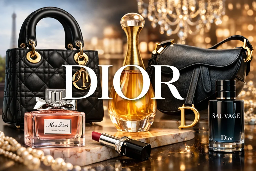
1. Lady Dior Bag
The Lady Dior handbag is one of Dior’s most iconic creations.
It became globally famous when Princess Diana was seen carrying it in the 1990s.
Features:
- Cannage stitching pattern
- Structured shape
- Dior letter charms
It remains one of the brand’s top-selling handbags.
2. Dior Saddle Bag
Designed by John Galliano in 1999, the Saddle Bag became a fashion icon.
- Unique curved shape
- Popular in early 2000s
- Revived successfully in 2018
Celebrities and influencers helped make it trendy again.
3. Miss Dior Perfume
Dior launched its first perfume, Miss Dior, in 1947.
It was named after Christian Dior’s sister, Catherine.
This fragrance symbolized femininity and romance.
Miss Dior remains one of the brand’s best-selling perfumes globally.
4. J’adore Dior
Another iconic fragrance is J’adore, launched in 1999.
Known for:
- Elegant golden bottle
- Floral fragrance
- Luxury marketing campaigns
It became one of the world’s most recognizable perfumes.
5. Dior Sauvage
In men’s fragrance, Sauvage became a massive global success.
It is often associated with actor Johnny Depp, who starred in its advertisements.
Sauvage is one of the best-selling men’s perfumes worldwide.
6. Dior Beauty & Makeup
Dior is also powerful in cosmetics, including:
- Dior Addict Lipstick
- Dior Forever Foundation
- Capture Totale Skincare
Dior Beauty contributes significantly to the company’s revenue.
Dior in Modern Fashion
Today, Dior stands for:
- Feminine power
- Artistic innovation
- Craftsmanship
- Luxury heritage
Under Maria Grazia Chiuri, Dior promotes feminism and empowerment through fashion slogans like:
“We Should All Be Feminists”
The brand blends tradition with modern social messages.
Financial Growth & Market Power
Dior is among the top luxury brands globally, competing with:
- Chanel
- Gucci
- Louis Vuitton
The company generates billions in annual revenue through fashion, accessories, and beauty products.
Its global presence includes:
- Flagship stores in Paris, New York, Dubai, London, and Tokyo
- Strong online luxury sales
- Celebrity endorsements
Timeline of Dior’s Major Milestones
- 1946 – Dior founded in Paris
- 1947 – New Look collection launched
- 1957 – Christian Dior passes away
- 1995 – Lady Dior bag becomes iconic
- 1999 – J’adore perfume launched
- 2000 – Saddle Bag becomes fashion trend
- 2016 – Maria Grazia Chiuri becomes first female creative director
- Present – Dior remains a global luxury powerhouse
Why Dior Remains Successful
Dior’s long-term success comes from:
- Strong brand identity
- Heritage and craftsmanship
- Iconic products
- Smart leadership under LVMH
- Continuous innovation
The brand respects its history while evolving with modern trends.
 1940s – The Beginning of Dior Fragrance
 1940s – The Beginning of Dior Fragrance
1947 – Miss Dior
The first Dior perfume was Miss Dior, created the same year as the “New Look” fashion collection.
- Named after Christian Dior’s sister Catherine.
- Elegant floral chypre fragrance.
- Symbolized femininity and post-war renewal.
- Became instantly successful.
This perfume established Dior as not just a fashion house — but also a fragrance powerhouse.
1950s – Expansion of Luxury Scents
 1950s – Expansion of Luxury Scents
1949 – Diorama
- Rich floral-fruity fragrance.
- Inspired by Dior’s love for gardens and nature.
1956 – Diorissimo
Created by legendary perfumer Edmond Roudnitska.
- Focused on lily-of-the-valley scent.
- Fresh, delicate, and romantic.
- Became one of Dior’s most artistic fragrances.
Diorissimo remains a classic in haute perfumery.
1960s – Modern Femininity
 1960s – Modern Femininity
1966 – Eau Sauvage
Created for men.
- Fresh citrus fragrance.
- Also developed by Edmond Roudnitska.
- Revolutionized men’s perfumery with elegance and simplicity.
Eau Sauvage became a timeless masculine fragrance and remains in production today.
1980s – Bold & Glamorous Era
 1980s – Bold & Glamorous Era
1985 – Poison
One of Dior’s most dramatic launches.
- Deep, spicy, mysterious scent.
- Purple bottle design.
- Very strong projection and lasting power.
Poison became a global bestseller and introduced a bold, seductive identity to Dior perfumes.
Later variations included:
- Tendre Poison
- Hypnotic Poison
- Pure Poison
1990s – Feminine Luxury & Global Expansion
 1990s – Feminine Luxury & Global Expansion
1991 – Dune
- Inspired by nature and sea breeze.
- Soft oriental fragrance.
- Calm, warm, and elegant.
1999 – J’adore
One of Dior’s biggest fragrance successes.
- Floral-fruity composition.
- Iconic gold amphora-shaped bottle.
- Represented modern femininity and luxury.
J’adore became one of the world’s best-selling perfumes and remains a major revenue driver for Dior.
2000s – Modern Icons
 2000s – Modern Icons
2002 – Dior Addict
- Sensual oriental fragrance.
- Dark blue bottle.
- Represented bold, confident women.
2005 – Miss Dior Chérie
- Youthful, sweet, romantic version of Miss Dior.
- Popular among younger consumers.
2006 – Dior Homme
- Powdery iris-based men’s fragrance.
- Elegant and artistic.
- Redefined men’s fragrance sophistication.
2010s – Global Commercial Success
 2010s – Global Commercial Success
2015 – Sauvage
One of Dior’s most successful perfumes ever.
- Fresh, spicy, woody fragrance.
- Massive global popularity.
- Marketed with actor Johnny Depp.
Sauvage became one of the best-selling men’s fragrances worldwide.
2017 – Miss Dior (Reformulations & Relaunches)
Miss Dior evolved several times:
- Lighter floral versions
- Modernized formulas
- Contemporary branding
The brand kept updating it to match modern tastes.
2018 – Joy by Dior
- Fresh floral fragrance.
- Promoted as a “joyful” everyday scent.
- Also associated with Johnny Depp in campaigns.
2020s – Luxury & Niche Direction
 2020s – Luxury & Niche Direction
2020 – J’adore Infinissime
- Stronger, richer version of J’adore.
- More sensual and intense.
2021 – Miss Dior (New Formula)
- Focus on sustainable ingredients.
- Modern rose-based scent.
2023 – Sauvage Elixir
- More concentrated and intense version of Sauvage.
- Extremely popular in global fragrance market.
Dior La Collection Privée (Luxury Line)
Dior also launched a premium niche line called:
La Collection Privée Christian Dior
- Exclusive luxury fragrances
- High-quality ingredients
- Sold in select boutiques
Popular scents include:
- Ambre Nuit
- Oud Ispahan
- Gris Dior
This collection targets luxury fragrance lovers.
Summary Timeline (Quick View)
| Year | Perfume | Significance |
|---|---|---|
| 1947 | Miss Dior | First fragrance |
| 1956 | Diorissimo | Classic floral |
| 1966 | Eau Sauvage | First iconic men’s scent |
| 1985 | Poison | Bold global hit |
| 1999 | J’adore | Worldwide bestseller |
| 2002 | Dior Addict | Sensual modern fragrance |
| 2006 | Dior Homme | Artistic men’s scent |
| 2015 | Sauvage | Massive global success |
| 2018 | Joy | Modern everyday fragrance |
| 2023 | Sauvage Elixir | Intense luxury version |
Why Dior Perfumes Are So Successful
- Strong brand heritage
- Collaboration with legendary perfumers
- Iconic bottle designs
- Celebrity marketing
- Continuous reformulation and modernization
Dior perfumes combine French elegance, artistic craftsmanship, and global marketing power.
From Miss Dior (1947) to Sauvage Elixir (2023), Dior perfumes have shaped the fragrance industry for nearly 80 years.
They reflect changing times — from post-war femininity to modern bold confidence — while always maintaining luxury and elegance.
Dior fragrances are not just perfumes; they are emotional experiences bottled in art.
For more readings;