Solved Paper Statistics for Business Decisions 2017 BMS CBCS Delhi University

In this post, I am going to present you the Solved Paper Statistics for Business Decisions 2017 BMS CBCS Delhi University for BMS Bachelor of Management Studies. Poisson Distribution, Rank Correlation Coefficient, Hypothesis, Measures of Central Tendency & Dispersion, Slicing are key requirements in this paper. Stay in touch for other study notes and solutions of the papers related to Statistics, Accounting, Finance, economics & other resource of Investment, Corporate finance and business.

bcfeducation.com

Solved by Iftikhar Ali Lecturer Business & Financial Studies

Solved Paper Statistics for Business Decisions 2017 BMS CBCS Delhi University

Q.1: (a) Listed below is frequency distribution for returns in percentage terms for a sample of 100 equity mutual funds for the year 2016-17……….Compare the cut-off point returns for the top 25% and the bottom 25% of the distribution. What are the average returns?

Q.1: (a) Listed below is frequency distribution for returns in percentage terms for a sample of 100 equity mutual funds for the year 2016-17.

*Returns%*	*Number of Mutual Funds (f)*
0—5	8
5—10	26
10—15	40
15—20	16
20—25	10

Compare the cut-off point returns for the top 25% and the bottom 25% of the distribution. What are the average returns? (6 Marks)

bcfeducation.com

Solution:

*Returns%*	X	*(f)*	*C.f*
0—5	2.5	8	8
5—10	7.5	26	34
10—15	12.5	40	74
15—20	17.5	16	90
20—25	22.5	10	100
		*∑f=n=100*

Bottom 25% cut-off point

25% of 100 = 25

25 ends before c.f 34 so cut-off point for bottom is 0—5

$\(Average\ for\ bottom = \frac{\frac{2.5}{8}}{8} = 2.5\%\$

Top 25% cut-off point

75% of 100 = 75 75 falls in c.f 90 but greater than c.f 74 so cut-off point for top is 15—20

$\(Average\ for\ Top = \frac{\frac{17.5}{8}}{8} = 17.5\%\$

(b) In a survey it was found that out of the total number of mobile phone owners, 35% are below the age group of 25 years and the remaining 65% above………Airtel connection. Given that a mobile phone owner is an Airtel subscriber. What is the likelihood that he/she is below 25 years of age?

(b) In a survey it was found that out of the total number of mobile phone owners, 35% are below the age group of 25 years and the remaining 65% above. Further, from another survey it was found that out of total number of mobile owners below 25 years of age, 40% are Airtel service subscribers. On the other hand 30% of above 25 years mobile owners have an Airtel connection. Given that a mobile phone owner is an Airtel subscriber. What is the likelihood that he/she is below 25 years of age? (5 Marks)

Solution:

Events:

Mobile phone owner is below 25 years of age = A

Mobile phone owner is an Airtel subscriber = B

Probability of mobile phone owner is below 25 years of age given that they are an Airtel subscriber = P(A|B)

Probability of a person is an Airtel subscriber below 25 years of age = P(B|A)

P(A) = 0.35

P(B) = (0.40)(0.35) + (0.30)(0.65) = 0.14 + 0.195 = 0.335

P(B|A) = 0.40

P(A|B) = ?

Apply Bayes Theorem

$\(\mathbf{P(A|B)\ =}\frac{\mathbf{P(B|A) \times P(A)\ }}{\mathbf{P(B)}}\$

$\(\mathbf{P(A|B)\ =}\frac{\mathbf{0.40 \times 0.35\ }}{\mathbf{0.335}}\$

$\(\mathbf{P}\left( \mathbf{A} \middle| \mathbf{B} \right)\mathbf{= 0.4179}\$

So, the likelihood that a mobile phone owner, who is an Airtel subscriber, is below 25 years of age is approximately 0.4179 or 41.79%

(c) Calculate the Fisher’s Index for the Year 2016 using the following data (with 2015 as the Base Year):

(c) Calculate the Fisher’s Index for the Year 2016 using the following data (with 2015 as the Base Year):

Commodity	2015	2015	2016	2016
	Price	Expenditure	Price	Expenditure
A	8	200	65	1950
B	20	1400	30	1650
C	5	80	20	900
D	10	360	15	300
E	27	2160	10	600

(4 Marks)

Solution:

Commodity	2015		2016		*poqo*	*p1q1*	*p1qo*	*poq1*
Commodity	*Price po*	*Expenditure q0*	*Price p1*	*Expenditure q1*
A	8	200/8=25	65	1950/65=30	200	1950	1625	240
B	20	1400/20=70	30	1650/30=55	1400	1650	2100	1100
C	5	80/5=16	20	900/20=45	80	900	320	225
D	10	360/10=36	15	300/15=20	360	300	540	200
E	27	2160/27=80	10	600/10=60	2160	600	800	1620
					4200	5400	5385	3385
					*∑poqo=*	*∑p1q1=*	*∑p1qo=*	*∑poq1=*

bcfeducation.com

$\(\mathbf{Fishe}\mathbf{r}^{\mathbf{'}}\mathbf{s\ Ideal\ Index\ 2016 =}\sqrt{\left( \frac{\mathbf{\sum}\mathbf{p}_{\mathbf{1}}\mathbf{q}_{\mathbf{o}}}{\mathbf{\sum}\mathbf{p}_{\mathbf{o}}\mathbf{q}_{\mathbf{o}}}\mathbf{\ \times \ }\frac{\mathbf{\sum}\mathbf{p}_{\mathbf{1}}\mathbf{q}_{\mathbf{1}}}{\mathbf{\sum}\mathbf{p}_{\mathbf{o}}\mathbf{q}_{\mathbf{1}}} \right)}\mathbf{\ \times \ 100}\$

$\(\mathbf{Fishe}\mathbf{r}^{\mathbf{'}}\mathbf{s\ Ideal\ Index\ 2016 =}\sqrt{\left( \frac{\mathbf{5385}}{\mathbf{4200}}\mathbf{\ \times \ }\frac{\mathbf{5400}}{\mathbf{3385}} \right)}\mathbf{\ \times \ 100}\$

$\(\mathbf{Fishe}\mathbf{r}^{\mathbf{'}}\mathbf{s\ Ideal\ Index\ 2016 =}\sqrt{\left( \mathbf{1.2821\ \times \ 1.5952} \right)}\mathbf{\ \times \ 100}\$

$\(\mathbf{Fishe}\mathbf{r}^{\mathbf{'}}\mathbf{s\ Ideal\ Index\ 2016 = 143}\$

Q.2: (a) A survey was conducted among college students to enquire how much they spent on eating out in the last one month. The following data was obtained……..What is the average monthly expenditure? Find the Karl Pearson’s coefficient of skewness.

Q.2: (a) A survey was conducted among college students to enquire how much they spent on eating out in the last one month. The following data was obtained:

*Expenditures*	*Number of Students*
0—50	20
50—100	10
100—150	25
150—200	20
200—250	10
250—500	15

What is the average monthly expenditure? Find the Karl Pearson’s coefficient of skewness. (6 Marks)

Solution:

*Expenditures*	f	X	fx	*fx²*
0—50	20	25	500	12500
50—100	10	75	750	56250
100—150	25	125	3125	390625
150—200	20	175	3500	612500
200—250	10	225	2250	506250
250—500	15	375	5625	2109375
	100		15750	3687500
	*∑f=*		*∑fx=*	*∑fx²=*

$\(\mathbf{Mean =}\frac{\mathbf{\sum fx}}{\mathbf{\sum f}}\mathbf{=}\frac{\mathbf{15750}}{\mathbf{100}}\mathbf{= 157.50}\$

$\(\mathbf{Mode = l +}\frac{\mathbf{fm - f}\mathbf{1}}{\left( \mathbf{fm - f}\mathbf{1} \right)\mathbf{+ (fm - f}\mathbf{2)}}\mathbf{\times h}\$

Maximum frequency is 25 so l=100, fm =25, f1 =10, f2 =20, h =50

$\(\mathbf{Mode = 100 +}\frac{\mathbf{25 - 10}}{\left( \mathbf{25 - 10} \right)\mathbf{+ (25 - 20)}}\mathbf{\times 50}\$

$\(\mathbf{Mode = 100 +}\frac{\mathbf{750}}{\mathbf{20}}\$

$\(\mathbf{Mode = 137.5}\$

$\(\mathbf{S.D =}\sqrt{\frac{\mathbf{\sum fx²}}{\mathbf{\sum f}}\mathbf{-}\left( \frac{\mathbf{\sum fx}}{\mathbf{\sum f}} \right)^{\mathbf{2}}}\$

$\(\mathbf{S.D =}\sqrt{\frac{\mathbf{3687500}}{\mathbf{100}}\mathbf{-}\left( \mathbf{157.50} \right)^{\mathbf{2}}}\$

$\(\mathbf{S.D =}\sqrt{\mathbf{36875 - 24806.25}}\$

$\(\mathbf{S.D = 109.85}\$

$\(\mathbf{Karl\ Pearson\ C.Skewness =}\frac{\mathbf{Mean - Mode}}{\mathbf{S.D}}\$

$\(\mathbf{Karl\ Pearson\ C.Skewness =}\frac{\mathbf{157.50 - 137.5}}{\mathbf{109.85}}\$

$\(\mathbf{Karl\ Pearson\ C.Skewness = 0.1820}\$

Positive Skewness longer tail to the right

(b) After an analysis of incoming faxes the manager of an accounting firm determined the probability distribution of the number of pages (X) per facsimile as follows………..Compute the mean and variance of the number of pages per fax. Further analysis by the manager revealed that the cost of processing each page of a fax is 0.25 Dollar. Determine the mean and variance of the cost per fax.

bcfeducation.com

(b) After an analysis of incoming faxes the manager of an accounting firm determined the probability distribution of the number of pages (X) per facsimile as follows:

X	1	2	3	4	5	6	7
P(x)	0.05	0.12	0.20	0.30	0.15	0.10	0.08

Compute the mean and variance of the number of pages per fax. Further analysis by the manager revealed that the cost of processing each page of a fax is 0.25 Dollar. Determine the mean and variance of the cost per fax. (5 Marks)

Solution:

x	*p(x)*	*xp(x)*	*x²p(x)*
1	0.05	0.05	0.05
2	0.12	0.24	0.48
3	0.2	0.6	1.8
4	0.3	1.2	4.8
5	0.15	0.75	3.75
6	0.1	0.6	3.6
7	0.08	0.56	3.92
		4	18.4
		∑ xp(x)=	∑ x²p(x)=

Mean=E(X) = ∑ xp(x) = 4

Variance (X) = E(X²) – E(X)²

Variance (X) = ∑ x²p(x) – [∑ xp(x)]²

Variance (X) = 18.4 – (4)²

Variance (X) = 2.4

Mean and variance of the cost per fax if processing cost is 0.25 Dollar:

Y = 0.25X

E(Y) = E(0.25X)

E(Y) = 0.25E(X)

E(Y) = 0.25(4)

Mean E(Y) = 1

V(Y) = V(0.25X)

V(Y) = (0.25)²Var(X)

V(Y) = (0.0625)(2.4)

V(Y) = 0.15

(c) Distinguish between Correlation and Regression analysis. (4 Marks)

Answer: While both regression and correlation analysis are statistical methods for examining quantifiable relationship between variables, they have distinct uses and provide various kinds of data:

Correlation Analysis:

Definition:

Correlation analysis is a statistical technique used to determine the direction and degree of a link between two quantitative variables.

Goal: Without suggesting causality, it aids in understanding how changes in one variable are related to changes in another.

Quantify: The coefficient of correlation, commonly represented as (r).

Measure: The degree of a linear relationship between two variables may be measured using correlation. It has a range of -1 to 1, with 0 denoting no linear correlation, -1 denoting perfect negative correlation, and 1 denoting perfect positive correlation.

Interpretation: A strong linear relationship is indicated by a correlation around -1 or 1, whereas a weak or nonexistent linear link is indicated by a correlation near 0.
For instance, correlation analysis may be used to look at the link between study time and test results or rainfall and agricultural productivity.

Regression Analysis:

Definition:

A statistical technique called regression analysis is used to describe the connection between one or more independent variables (predictors) and a dependent variable (response).

Goal: It is useful to comprehend the nature of the relationship between the independent and dependent variables and to forecast the value of the dependent variable based on the values of the independent variables.

Models: Depending on the characteristics of the variables and the relationship’s underlying assumptions, there are several kinds of regression models, including logistic regression, multiple regression, and linear regression.

Measure: The coefficients in the regression equation show the strength and direction of each independent variable’s influence on the dependent variable. The regression equation depicts the mathematical link between the variables.

bcfeducation.com

Interpretation: Regression analysis enables prediction and hypothesis testing while offering insights into how changes in one or more independent variables impact the dependent variable.
For instance, regression analysis may be used to estimate the link between temperature and ice cream sales or to anticipate property values based on variables like size, location, and number of bedrooms.

In conclusion, regression analysis models the link between a dependent variable and one or more independent variables, enabling prediction and hypothesis testing, whereas correlation analysis measures the strength and direction of the association between two variables. While they accomplish distinct goals in terms of comprehending the connections between variables, both approaches are useful tools for data analysis and interpretation.

Q.3: (a) The table given below provides a summary of total; expenditure by the Government of India for Health and Sanitation from 2010-11 to 2016-17……..Fit an exponential trend (Y = a+bx) to the given data and estimate the expenditure for the year 2017-18.

Q.3: (a) The table given below provides a summary of total; expenditure by the Government of India for Health and Sanitation from 2010-11 to 2016-17:

Year	2010-11	2011-12	2012-13	2013-14	2014-15	2015-16	2016-17
Expenditure (in Rs. Crore)	177.2	185.0	224.9	254.0	304.9	359.9	438.8

Fit an exponential trend (Y = a+bx) to the given data and estimate the expenditure for the year 2017-18. (6 Marks)

Solution:

*Year*	*Expenditures (in Rs. Crore) Steel (m.t) (y)*	*x = t – 2012*	x²	xy
2010-11	177.2	-3	9	-531.6
2011-12	185	-2	4	-370
2012-13	224.9	-1	1	-224.9
2013-14	254	0	0	0
2014-15	304.9	1	1	304.9
2015-16	359.9	2	4	719.8
2016-17	438.8	3	9	1316.4
*n=7*	*∑y =1944.7*	*∑x = 0*	*∑x² = 28*	*∑xy =1214.6*

Fitting straight Line

Let the straight line:

y = a + bx where

$\(\mathbf{a =}\frac{\mathbf{\sum y}}{\mathbf{n}}\mathbf{,\ b =}\frac{\mathbf{\sum xy}}{\mathbf{\sum}\mathbf{x}^{\mathbf{2}}}\$

$\(\mathbf{a =}\frac{\mathbf{\sum y}}{\mathbf{n}}\mathbf{=}\frac{\mathbf{1944.7}}{\mathbf{7}}\mathbf{= 277.81}\$

$\(\mathbf{b =}\frac{\mathbf{\sum xy}}{\mathbf{\sum}\mathbf{x}^{\mathbf{2}}}\mathbf{=}\frac{\mathbf{1214.6}}{\mathbf{28}}\mathbf{= 43.3785}\$

y = a + bx

y = 277.81 + 43.3785x

Estimate the expenditure for the year 20l7-18

First x = t – 2017-18 = 4

Now putting x = 4 into straight line equation:

y = 277.81 + 43.3785x

y = 277.81 + 43.3785(4)

y = 451.324 so the expenditure for the year 2017-18 will be 451.324.

(b) Given below are the approximate average returns obtained from Gold and real estate over the last 5 years………………..Which of the two offers the more consistent returns?

(b) Given below are the approximate average returns obtained from Gold and real estate over the last 5 years:

Year	Gold %	Real Estate %
2012-13	10	8
2013-14	10	7
2014-15	6	5
2015-16	4	5
2016-17	9	3

Which of the two offers the more consistent returns? (5 Marks)

Solution:

Year	*Gold % (X1)*	*X1²*	*Real Estate %(X2)*	*X2²*
2012-13	10	100	8	64
2013-14	10	100	7	49
2014-15	6	36	5	25
2015-16	4	16	5	25
2016-17	9	81	3	9

	∑ X1 =39	∑ X1²=333	∑ X2 =28	∑ X2²=172

Mean & C.V of Gold:

$\({\overline{\mathbf{X}}}_{\mathbf{Gold}}\mathbf{=}\frac{\mathbf{\sum x}\mathbf{1}}{\mathbf{n}\mathbf{1}}\$

$\({\overline{\mathbf{X}}}_{\mathbf{Gold}}\mathbf{=}\frac{\mathbf{39}}{\mathbf{5}}\mathbf{= 7.8}\$

$\(\mathbf{S.D\ Gold =}\sqrt{\frac{\mathbf{\sum x}\mathbf{1}^{\mathbf{2}}}{\mathbf{n}\mathbf{1}}\mathbf{-}\left( \frac{\mathbf{\sum x}\mathbf{1}}{\mathbf{n}\mathbf{1}} \right)^{\mathbf{2}}}\$

$\(\mathbf{S.D\ Gold =}\sqrt{\frac{\mathbf{333}}{\mathbf{5}}\mathbf{-}\left( \mathbf{7.8} \right)^{\mathbf{2}}}\$

$\(\mathbf{S.D\ Gold =}\sqrt{\mathbf{5.76}}\$

$\(\mathbf{S.D\ Gold = 2.4}\$

$\(\mathbf{C.V\ Gold =}\frac{\mathbf{\ S.D}}{\mathbf{Mean}}\mathbf{\times 100}\$

$\(\mathbf{C.V\ Gold =}\frac{\mathbf{\ 2.4}}{\mathbf{7.8}}\mathbf{\times 100}\$

$\(\mathbf{C.V\ Gold = 30.76}\$

Mean & C.V of Real Estate:

$\({\overline{\mathbf{X}}}_{\mathbf{Real\ Estate}}\mathbf{=}\frac{\mathbf{\sum x}\mathbf{2}}{\mathbf{n}\mathbf{2}}\$

$\({\overline{\mathbf{X}}}_{\mathbf{Real\ Estate}}\mathbf{=}\frac{\mathbf{28}}{\mathbf{5}}\mathbf{= 5.6}\$

$\(\mathbf{S.D\ Real\ Estate =}\sqrt{\frac{\mathbf{\sum x}\mathbf{2}^{\mathbf{2}}}{\mathbf{n}\mathbf{2}}\mathbf{-}\left( \frac{\mathbf{\sum x}\mathbf{2}}{\mathbf{n}\mathbf{2}} \right)^{\mathbf{2}}}\$

$\(\mathbf{S.D\ Real\ Estate =}\sqrt{\frac{\mathbf{172}}{\mathbf{5}}\mathbf{-}\left( \mathbf{5.6} \right)^{\mathbf{2}}}\$

$\(\mathbf{S.D\ Real\ Estate =}\sqrt{\mathbf{3.04}}\$

$\(\mathbf{S.D\ Real\ Estate = 1.7435}\$

$\(\mathbf{C.V\ Real\ Estate =}\frac{\mathbf{\ S.D}}{\mathbf{Mean}}\mathbf{\times 100}\$

$\(\mathbf{C.V\ Real\ Estate =}\frac{\mathbf{\ 1.7435}}{\mathbf{5.6}}\mathbf{\times 100}\$

$\(\mathbf{C.V\ Real\ Estate = 31.13}\$

bcfeducation.com

Results:

Gold Mean = 7.8

Gold C.V = 30.76%

Real Estate Mean = 5.6

Real Estate C.V = 31.13%

Conclusion:

Average return of Gold 7.8% is greater than the average return of Real Estate 5.6% so Gold has higher return than real estate.

C.V of Gold 30.76% is less than the C.V of Real Estate 31.13% so Gold stock is more consistent than Real Estate.

(c) A manufacturing company regularly conducts quality control checks at specified periods on the products it manufactures. Historically, the failure rate for LED light bulbs that the company manufactures is 5%. Suppose a random sample of 10 LED bulbs is selected. Let X represents number of defective LED light bulbs.

(i) What is the probability that two or fewer of the LED light bulbs are defective?

(ii) What is the mean and variance of X? (4 Marks)

Solution:

(i) What is the probability that two or fewer of the LED light bulbs are defective?

Here our concern is to check the probability of defective bulbs so we select p = 0.05 and q = 0.95

$\(\mathbf{p = 0.05,\ q = 0.95}\$

$\(\mathbf{n = 10,\ x = 0,1,2,3,4,5,6,7,8,9,10}\$

Formula

$\(\mathbf{P}\left( \mathbf{X = x} \right)\mathbf{=}\begin{pmatrix} \mathbf{n} \\ \mathbf{x} \\ \end{pmatrix}\mathbf{\ }\mathbf{p}^{\mathbf{x}}\mathbf{\ }\mathbf{q}^{\mathbf{n - x}}\$

$\(\mathbf{P}\left( \mathbf{X = 2} \right)\mathbf{=}\begin{pmatrix} \mathbf{10} \\ \mathbf{2} \\ \end{pmatrix}\mathbf{\ }\left( \mathbf{0.05} \right)^{\mathbf{2}}\mathbf{\ }\left( \mathbf{0.95} \right)^{\mathbf{10 - 2}}\$

$\(\mathbf{P}\left( \mathbf{X = 2} \right)\mathbf{= 45 \times 0.0025 \times 0.6634 = 0.0746}\$

$\(\mathbf{P}\left( \mathbf{X = 1} \right)\mathbf{=}\begin{pmatrix} \mathbf{10} \\ \mathbf{1} \\ \end{pmatrix}\mathbf{\ }\left( \mathbf{0.05} \right)^{\mathbf{1}}\mathbf{\ }\left( \mathbf{0.95} \right)^{\mathbf{10 - 1}}\$

$\(\mathbf{P}\left( \mathbf{X = 1} \right)\mathbf{= 10 \times 0.05 \times 0.6302 = 0.3151}\$

$\(\mathbf{P}\left( \mathbf{X = 0} \right)\mathbf{=}\begin{pmatrix} \mathbf{10} \\ \mathbf{0} \\ \end{pmatrix}\mathbf{\ }\left( \mathbf{0.05} \right)^{\mathbf{0}}\mathbf{\ }\left( \mathbf{0.95} \right)^{\mathbf{10 - 0}}\$

$\(\mathbf{P}\left( \mathbf{X = 0} \right)\mathbf{= 1 \times 1 \times 0.5987 = 0.5987}\$

$\(\mathbf{P}\left( \mathbf{X \leq 2} \right)\mathbf{= 0.5987}\mathbf{+}\mathbf{0.3151 + 0.0746 = 0.9884}\$

(ii) What is the mean and variance of X?

Mean = np

Mean = (10)(0.05)=0.5

Variance = npq

Variance = (10)(0.05)(0.95)Variance =0.475

Q.4: (a) The following data relates to scores obtained by nine Salesmen of a company in an Intelligence test and their Weekly Sales (in ‘000)………..Obtain the two regression equations; Weekly Sales on Intelligence test score of the Salesman and Intelligence test score of the Sales man on Weekly Sales . If the Intelligence test score of a Sales man is 65, what would be his expected Weekly Sales?

Q.4: (a) The following data relates to scores obtained by nine Salesmen of a company in an Intelligence test and their Weekly Sales (in ‘000):

Salesman	Test Score	Weekly Sales (in “1000”)
1	50	30
2	60	60
3	50	40
4	60	50
5	80	60
6	50	30
7	80	70
8	40	50
9	70	60

Obtain the two regression equations; Weekly Sales on Intelligence test score of the Salesman and Intelligence test score of the Sales man on Weekly Sales . If the Intelligence test score of a Sales man is 65, what would be his expected Weekly Sales? (6 Marks)

Solution:

*Test Score (X)*	*Weekly Sales (in “1000”) (Y)*	XY	X²	Y²
50	30	1500	2500	900
60	60	3600	3600	3600
50	40	2000	2500	1600
60	50	3000	3600	2500
80	60	4800	6400	3600
50	30	1500	2500	900
80	70	5600	6400	4900
40	50	2000	1600	2500
70	60	4200	4900	3600
*540*	*450*	*28200*	*34000*	*24100*
*∑x =*	*∑y =*	*∑xy =*	*∑x² =*	*∑y² =*

Line of Regression Y on X Weekly Sales on Intelligence test score of the Salesman

$\(\widehat{\mathbf{Y}}\mathbf{= a + bx}\$

Where:

$\(\mathbf{a =}\overline{\mathbf{Y}}\mathbf{- b}\overline{\mathbf{X}}\mathbf{\ \ \&\ }\mathbf{b}_{\mathbf{yx}}\mathbf{=}\frac{\mathbf{\sum xy - n}\overline{\mathbf{X}}\overline{\mathbf{Y}}}{\mathbf{\sum}\mathbf{x}^{\mathbf{2}}\mathbf{- n}{\mathbf{(}\overline{\mathbf{X}}\mathbf{)}}^{\mathbf{2}}}\mathbf{\ \ \ }\$

$\(\overline{\mathbf{X}}\mathbf{=}\frac{\mathbf{\sum x}}{\mathbf{n}}\mathbf{=}\frac{\mathbf{540}}{\mathbf{9}}\mathbf{= 60}\$

$\(\overline{\mathbf{Y}}\mathbf{=}\frac{\mathbf{\sum y}}{\mathbf{n}}\mathbf{=}\frac{\mathbf{450}}{\mathbf{9}}\mathbf{= 50}\$

$\(\mathbf{b}_{\mathbf{yx}}\mathbf{=}\frac{\mathbf{\sum xy - n}\overline{\mathbf{X}}\overline{\mathbf{Y}}}{\mathbf{\sum}\mathbf{x}^{\mathbf{2}}\mathbf{- n}{\mathbf{(}\overline{\mathbf{X}}\mathbf{)}}^{\mathbf{2}}}\mathbf{\ \ \ }\$

$\(\mathbf{b}_{\mathbf{yx}}\mathbf{=}\frac{\mathbf{28200 - 9(60)(50)}}{\mathbf{34000}\mathbf{- 9}\mathbf{(60)}^{\mathbf{2}}}\mathbf{\ \ \ }\$

$\(\mathbf{b}_{\mathbf{yx}}\mathbf{=}\frac{\mathbf{1200}}{\mathbf{1600}}\mathbf{= 0.75\ \ }\$

$\(\mathbf{a =}\overline{\mathbf{Y}}\mathbf{- b}\overline{\mathbf{X}}\$

$\(\mathbf{a = 50 - (0.75)(60)}\$

$\(\mathbf{a = 5}\$

$\(\widehat{\mathbf{Y}}\mathbf{= a + bx}\$

$\(\widehat{\mathbf{Y}}\mathbf{= 5 + 0.75}\mathbf{x}\$

Line of Regression X on Y Intelligence test score of the Sales man on Weekly Sales

$\(\widehat{\mathbf{X}}\mathbf{= a + by}\$

Where:

$\(\mathbf{a =}\overline{\mathbf{X}}\mathbf{- b}\overline{\mathbf{Y}}\mathbf{\ \ \&\ }\mathbf{b}_{\mathbf{xy}}\mathbf{=}\frac{\mathbf{\sum xy - n}\overline{\mathbf{X}}\overline{\mathbf{Y}}}{\mathbf{\sum}\mathbf{y}^{\mathbf{2}}\mathbf{- n}{\mathbf{(}\overline{\mathbf{Y}}\mathbf{)}}^{\mathbf{2}}}\$

$\(\mathbf{b}_{\mathbf{xy}}\mathbf{=}\frac{\mathbf{\sum xy - n}\overline{\mathbf{X}}\overline{\mathbf{Y}}}{\mathbf{\sum}\mathbf{y}^{\mathbf{2}}\mathbf{- n}{\mathbf{(}\overline{\mathbf{Y}}\mathbf{)}}^{\mathbf{2}}}\$

$\(\mathbf{b}_{\mathbf{xy}}\mathbf{=}\frac{\mathbf{28200 - 9(60)(50)}}{\mathbf{24100 - 9}\mathbf{(50)}^{\mathbf{2}}}\$

$\(\mathbf{b}_{\mathbf{xy}}\mathbf{=}\frac{\mathbf{1200}}{\mathbf{1600}}\mathbf{= 0.75}\$

$\(\mathbf{a =}\overline{\mathbf{X}}\mathbf{- b}\overline{\mathbf{Y}}\$

$\(\mathbf{a = 60 - 0.75(50)}\$

$\(\mathbf{a = 22.5}\$

$\(\widehat{\mathbf{X}}\mathbf{= a + by}\$

$\(\widehat{\mathbf{X}}\mathbf{= 22.5 + 0.75}\mathbf{y}\$

If the Intelligence test score of a Sales man is 65, what would be his expected Weekly Sales?

$\(\widehat{\mathbf{Y}}\mathbf{= 5 + 0.75}\mathbf{x}\$

$\(\widehat{\mathbf{Y}}\mathbf{= 5 + 0.75(65)}\$

$\(\widehat{\mathbf{Y}}\mathbf{= 53.75}\$

bcfeducation.com

(b) ABC Trucking Company determined that the distance travelled per truck per year is normally distributed, with a mean of 50 thousand miles and a standard deviation of 12 thousand miles.

(i) What proportion of trucks can be expected to travel between 34 and 50 thousand miles in a year?

(ii) How many miles will be travelled by at least 80% of the trucks? (5 Marks)

Solution: (i)

$\(\mathbf{Z}_{\mathbf{1}}\mathbf{=}\frac{\mathbf{X - Mu}}{\mathbf{\sigma}}\mathbf{=}\frac{\mathbf{34000 - 50000}}{\mathbf{12000}}\mathbf{= - 1.33}\$

$\(\mathbf{Z}_{\mathbf{2}}\mathbf{=}\frac{\mathbf{X - Mu}}{\mathbf{\sigma}}\mathbf{=}\frac{\mathbf{50000 - 50000}}{\mathbf{12000}}\mathbf{= 0}\$

$\(\mathbf{P}\left( \mathbf{34000 < X < 50000} \right)\mathbf{= P( - 1.33 < X < 0)}\$

Go to Z distribution table & find following probabilities:

$\(\mathbf{P}\left( \mathbf{- 1.33} \right)\mathbf{= 0.0918}\$

$\(\mathbf{P}\left( \mathbf{0} \right)\mathbf{= 0.5000}\$

Subtract above probabilities

0.5000 – 0.0918 = 0.4082

So 40.82% trucks can be expected to travel between 38 and 50 thousand miles in a year.

(ii) First we go to the Z Normal Probability Table and locate 1 – 0.80 =0.20 that will be found in -0.8 row and 4^th column.

So:

$\(Z_{0.80} = - 0.84,\ Mu = 50,000,\ \sigma = 12,000,\ X = ?\$

Formula Applied

$\(\mathbf{Z}_{\mathbf{0.80}}\mathbf{=}\frac{\mathbf{X - Mu}}{\mathbf{\sigma}}\$

$\(\mathbf{- 0.84 =}\frac{\mathbf{X - 50000}}{\mathbf{12000}}\$

$\(\mathbf{- 0.84 \times 12000 = X - 50000}\$

$\(\mathbf{X = - 10080 + 50000}\$

$\(\mathbf{X = 39920}\$

(c) Distinguish between Type I and Type II errors. (4 Marks)

Answer:

Type I Error:

Definition: False positives, or type I errors, happen when the null hypothesis (H0) is mistakenly rejected when it is true.
Probability: The likelihood of committing a Type I mistake, represented by 𝛼, indicates the test’s significance level.
Consequence: Making the wrong judgments by concluding that there is a major influence or difference when there isn’t.
Example: Dismissing the null hypothesis that a novel medication has no adverse effects when, in reality, none exist.

Type II Error:

Definition: False negatives, or type II errors, happen when the null hypothesis (H0) is mistakenly accepted when it is not, as is the case with this instance.
Probability: The likelihood of committing a Type II mistake is represented by 𝛽.
Consequence: Missing chances or drawing the wrong conclusions as a result of failing to identify a substantial influence or difference when there is one.
Example: Failing to reject the null hypothesis that a new medication has no adverse effects, when, in reality, it does.

Solution:

Data

X̅1 = 13.8, n1 = 41, S1 =18.9, S1² =357.21

X̅2 = 9.1, n2 = 35, S2 =8.7, S2² = 75.69

Step 1: Stating Null and Alternative Hypothesis

Ho: Null Hypotheses = µ1= µ2

H1: Alternative Hypotheses = µ1< µ2

Step 2: Level of significance

Alpha α = 0.05

Step 3: Test Statistics

$\(\mathbf{Z =}\frac{\mathbf{(x\overline{}}_{\mathbf{1}}\mathbf{-}{\overline{\mathbf{x}}}_{\mathbf{2)}}\mathbf{-}\mathbf{(\mu}_{\mathbf{1}}\mathbf{-}\mathbf{\mu}_{\mathbf{2}}\mathbf{)}}{\sqrt{\left( \frac{\mathbf{S}\mathbf{1}^{\mathbf{2}}}{\mathbf{n}_{\mathbf{1}}}\mathbf{+}\frac{\mathbf{S}\mathbf{2}^{\mathbf{2}}}{\mathbf{n}_{\mathbf{2}}} \right)}}\$

Step 4: Critical Region

1-0.05 = 0.95 go to Z Cumulative Standardized Normal Distribution Table & locate 0.95 Z > 1.645

$\(\mathbf{Z}_{\mathbf{\alpha}}\mathbf{=}\mathbf{Z}_{\mathbf{0.05}}\mathbf{= \pm 1.645)}\$

Step 5: Calculation

$\(\mathbf{Z =}\frac{\mathbf{13.8 - 9.1 - (0)}}{\sqrt{\left( \frac{\mathbf{357.21}}{\mathbf{41}}\mathbf{+}\frac{\mathbf{75.69}}{\mathbf{35}} \right)}}\$

$\(\mathbf{Z =}\frac{\mathbf{4.7}}{\mathbf{3.297}}\mathbf{= 1.425}\$

Step 6: Conclusion

Since calculated value of z statistic 1.425 is less than the tabulated value 1.645 or it falls in acceptance region so we accept null hypothesis and reject alternative hypothesis and we can conclude that at 5% level of significance FASB proposal will cause no reduction in EPS for high technology firms than for producers of consumer goods.

bcfeducation.com

(b) An economist wanted to find out whether there is any relationship between the unemployment rate in country and its inflation rate. Data from 7 countries for the year 2016 is given below……………………Use Spearman’s Rank Correlation to find the strength of association between unemployment rate in a country and its inflation rate.

(b) An economist wanted to find out whether there is any relationship between the unemployment rate in country and its inflation rate. Data from 7 countries for the year 2016 is given below:

Country	A	B	C	D	E	F	G
Unemployment rate (per cent)	11	9	13	7	13	8	8
Inflation rate (per cent)	4	5	7	8	6	3	5

Use Spearman’s Rank Correlation to find the strength of association between unemployment rate in a country and its inflation rate. (5 Marks)

Solution:

*Country*	*Unemployment rate (per cent)*	*Inflation rate (per cent)*	*Rank Unemployment Rate (x)*	*Rank Inflation Rate (y)*	*d=x-y*	d²
A	11	4	5	2	3	9
B	9	5	4	3.5	0.5	0.25
C	13	7	6.5	6	0.5	0.25
D	7	8	1	7	-6	36
E	13	6	6.5	5	1.5	2.25
F	8	3	2.5	1	1.5	2.25
G	8	5	2.5	3.5	-1	1
	n=7				*∑d=0*	*∑d²=51*

Hence, we see that in the X-series the items 8 and 13 are repeated, each occurring twice and in the

Y-series the item 5 is repeated. Thus in each of the three cases m = 2. We have to apply correction factor:

$\(Correction\ Factor = \ \frac{m(m^{2} - 1)}{12}\$

$\(Correction\ Factor = \ \frac{2(2^{2} - 1)}{12} + \frac{2(2^{2} - 1)}{12} + \frac{2(2^{2} - 1)}{12} = 1.5\$

$\(\rho_{xy} = 1 - \frac{6\sum d^{2}}{n(n^{2} - 1)}\$

But we have correction factor here so we are going to change the formula:

$\(\rho_{xy} = 1 - \frac{6\sum d^{2} + C.F}{n(n^{2} - 1)}\$

$\(\rho_{xy} = 1 - \frac{6(51) + 1.5}{7(7^{2} - 1)}\$

$\(\rho_{xy} = 1 - \frac{307.5}{336}\$

$\(\rho_{xy} = 0.0848\$

Indicating strong association

(c) A.B. Power and Associates calculates and publishes various statistics concerning car quality. The initial quality score measures the number of problems per new car sold. For 2017 model cars, an automobile company KPS had 1.02 problems per car. Let the random variable X be equal to the number of problems with a newly purchased 2017 KPS car.

(i) What assumptions must be made in order for X to be distributed as a Poisson random variable? Are these assumptions reasonable?

(ii) Making the assumptions as in (i), if you purchased a 2017 KPS car, what is the probability that the new car will have two or fewer problems? (4 Marks)

Solution:

(i) For the random variable X to be distributed as a Poisson random variable, several assumptions must be met:

The number of events (problems in this case) must be countable.

The events must occur independently of each other.

The probability of more than one event occurring in an infinitesimally small time interval is negligible.

The probability of an event occurring is constant over time and across all intervals.

In this case, assuming that each car’s problems are independent events and occur randomly with a constant average rate, the Poisson distribution could be a reasonable approximation.

(ii) Given that the average rate is 1.02 problems per car, we can use the Poisson distribution formula to find the probability of having two or fewer problems:

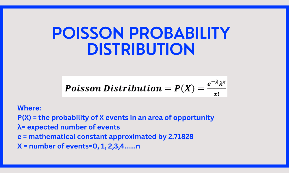
$\(\mathbf{Poisson\ Distribution = P}\left( \mathbf{X} \right)\mathbf{=}\frac{\mathbf{e}^{\mathbf{- \lambda}}\mathbf{\lambda}^{\mathbf{x}}}{\mathbf{x!}}\$

Where:

P(X) = the probability of X events in an area of opportunity

λ= expected number of events = 1.02

e = mathematical constant approximated by 2.71828

X = number of events=0, 1, 2

P(X=≤2)=P(x=1)+P(x=2)+P(x=3)

$\(\mathbf{P}\left( \mathbf{x = 0} \right)\mathbf{=}\frac{\left( \mathbf{2.71828} \right)^{\mathbf{- 1.02}}\mathbf{(1.02)}^{\mathbf{0}}}{\mathbf{0!}}\mathbf{= 0.36060}\$

$\(\mathbf{P}\left( \mathbf{x = 1} \right)\mathbf{=}\frac{\left( \mathbf{2.71828} \right)^{\mathbf{- 1.02}}\mathbf{(1.02)}^{\mathbf{1}}}{\mathbf{1!}}\mathbf{= 0.36781}\$

$\(\mathbf{P}\left( \mathbf{x = 2} \right)\mathbf{=}\frac{\left( \mathbf{2.71828} \right)^{\mathbf{- 1.02}}\mathbf{(1.02)}^{\mathbf{2}}}{\mathbf{2!}}\mathbf{= 0.18758}\$

P(X=≤2)= 0.36060+0.36781+0.18758 =0.91599

Q.6: (a) Prices of shares (in rupees) of a company on the different days in a month were found to be: 66, 65, 69, 70, 69, 71, 70, 63, 64 and 68. Assuming the prices of shares follow normal distribution and its standard distribution is unknown, test at 5 percent level of significance that the sample average price of the shares in that month is same as 65. Does the above data indicate that there is a factual basis for the grumblings? State and test appropriate hypothesis at alpha = 0.05? (6 Marks)

Solution:

Prices of Shares X	(X – X̅)	(X – X̅)²
66	-1.5	2.25
65	-2.5	6.25
69	1.5	2.25
70	2.5	6.25
69	1.5	2.25
71	3.5	12.25
70	2.5	6.25
63	-4.5	20.25
64	-3.5	12.25
68	0.5	0.25
*∑X=675*		∑(X – X̅)²=70.5

$\(\overline{\mathbf{X}}\mathbf{=}\frac{\mathbf{\sum X}}{\mathbf{n}}\mathbf{=}\frac{\mathbf{675}}{\mathbf{10}}\mathbf{= 67.5}\$

$\(\mathbf{S =}\sqrt{\frac{\mathbf{1}}{\mathbf{n - 1}}\mathbf{\sum}\left( \mathbf{X -}\overline{\mathbf{X}} \right)^{\mathbf{2}}}\$

$\(\mathbf{S =}\sqrt{\frac{\mathbf{1}}{\mathbf{10 - 1}}\mathbf{(70.5)}}\$

$\(\mathbf{S = 2.798}\$

Step 1: Stating Null and Alternative Hypothesis

Ho: Null Hypotheses = µ=65

H1: Alternative Hypotheses = µ ≠ 65

Step 2: Level of significance

Alpha α = 0.05, n = 10

Step 3: Test Statistics

$\(\mathbf{t =}\frac{\overline{\mathbf{x}}\mathbf{-}\mathbf{\mu}_{\mathbf{0}}}{\frac{\mathbf{s}}{\sqrt{\mathbf{n}}}}\$

Step 4: Critical Region

$\(\mathbf{t}_{\mathbf{0.05(10 - 1)}}\mathbf{= \pm 2.262}\$

$\(\mathbf{t\ > \ 2.262\ (t < 2.262\ and\ t > 2.262)}\$

Step 5: Calculation

$\(\mathbf{t =}\frac{\overline{\mathbf{x}}\mathbf{-}\mathbf{\mu}_{\mathbf{0}}}{\frac{\mathbf{s}}{\sqrt{\mathbf{n}}}}\$

$\(\mathbf{t =}\frac{\mathbf{67.5 - 65}}{\frac{\mathbf{2.798}}{\sqrt{\mathbf{10}}}}\$

$\(\mathbf{t =}\frac{\mathbf{2.5}}{\mathbf{0.8848}}\mathbf{= 2.8254}\$

Step 6: Conclusion

Since calculated value of t statistic 2.8254 exceeds than the tabulated value 2.262 or it falls in critical region so we reject null hypothesis and accept alternative hypothesis and we can say that the average price of the shares in that month is not same as 65.

Does the above data indicate that there is a factual basis for the grumblings?

Rejecting the null hypothesis indicates that there is enough data to draw the conclusion that the sample average share price differs considerably from 65 rupees. This does not, however, directly suggest whether or not the complaints have a solid basis in reality.

The null hypothesis is rejected, implying that the sample data indicates a different mean share price than 65 rupees. Depending on the situation and the specifics of the complaints, this may or may not validate the complaints.

If the complaints are about the share price being too high or too low in relation to an expected value (such as 65 rupees), then the null hypothesis’ rejection may validate such complaints. However, this statistical test by itself might not be sufficient to support or refute complaints regarding other factors unrelated to the mean share price.

In conclusion, even though the null hypothesis was rejected, there is still a difference in the sample mean share price. However, more research and context-specific considerations are required to ascertain whether the complaints have a solid foundation.

bcfeducation.com

(b) Given that the mean sale of 30 FMCG companies in the year 2016-17 was 300 crore and the mean sales of 70 IT companies was 2000 crore. The standard deviation for FMCG companies was, 50 crores and for IT companies 1000 crores. Find the combined mean and standard deviation for the two groups taken together. (5 Marks)

Solution:

Data Company A:

$\({\overline{\mathbf{X}}}_{\mathbf{FMCG}}\mathbf{= 300,\ }{\overline{\mathbf{X}}}_{\mathbf{IT}}\mathbf{= 2000}\$

$\(\mathbf{S}_{\mathbf{(FMCG)}}\mathbf{= 50,\ }\mathbf{S}_{\mathbf{(IT)}}\mathbf{= 1000}\$

$\({\mathbf{S}^{\mathbf{2}}}_{\mathbf{(FMCG)}}\mathbf{= 2500,\ }{\mathbf{S}^{\mathbf{2}}}_{\mathbf{(IT)}}\mathbf{= 1000,000}\$

$\(\mathbf{n}_{\mathbf{FMCG}}\mathbf{= 30,\ }\mathbf{n}_{\mathbf{IT}}\mathbf{= 70}\$

$\({\overline{\mathbf{X}}}_{\mathbf{c}}\mathbf{=}\frac{\mathbf{n}_{\mathbf{FMCG}}{\overline{\mathbf{X}}}_{\mathbf{FMCG}}\mathbf{+}\mathbf{n}_{\mathbf{IT}}{\overline{\mathbf{X}}}_{\mathbf{IT}}}{\mathbf{n}_{\mathbf{FMCG}}\mathbf{+}\mathbf{n}_{\mathbf{IT}}}\$

$\({\overline{\mathbf{X}}}_{\mathbf{c}}\mathbf{=}\frac{\mathbf{(30 \times 300) + (70 \times 2000)}}{\mathbf{30 + 70}}\$

$\({\overline{\mathbf{X}}}_{\mathbf{c}}\mathbf{=}\frac{\mathbf{9000 + 140000}}{\mathbf{100}}\$

$\({\overline{\mathbf{X}}}_{\mathbf{c}}\mathbf{= 1490}\$

$\(\mathbf{Combined\ S.D =}\sqrt{\frac{\mathbf{n}_{\mathbf{FMCG}}\left\lbrack {\mathbf{S}^{\mathbf{2}}}_{\mathbf{(FMCG)}}\mathbf{+}{\mathbf{(}{\overline{\mathbf{X}}}_{\mathbf{FMCG}}\mathbf{-}{\overline{\mathbf{X}}}_{\mathbf{c}}\mathbf{)}}^{\mathbf{2}} \right\rbrack\mathbf{+}\mathbf{n}_{\mathbf{IT}}\left\lbrack {\mathbf{S}^{\mathbf{2}}}_{\mathbf{(IT)}}\mathbf{+}{\mathbf{(}{\overline{\mathbf{X}}}_{\mathbf{IT}}\mathbf{-}{\overline{\mathbf{X}}}_{\mathbf{c}}\mathbf{)}}^{\mathbf{2}} \right\rbrack\mathbf{\ }}{\mathbf{n}_{\mathbf{FMCG}}\mathbf{+}\mathbf{n}_{\mathbf{IT}}}}\$

$\(\mathbf{Combined\ S.D =}\sqrt{\frac{\mathbf{30}\left\lbrack \mathbf{2500 +}\mathbf{(300 - 1490)}^{\mathbf{2}} \right\rbrack\mathbf{+ 70}\left\lbrack \mathbf{1000000 +}\mathbf{(2000 - 1490)}^{\mathbf{2}} \right\rbrack\mathbf{\ }}{\mathbf{30 + 70}}}\$

$\(\mathbf{Combined\ S.D =}\sqrt{\frac{\mathbf{42558000 + 88207000\ }}{\mathbf{100}}}\$

$\(\mathbf{Combined\ S.D = 1143.52}\$

$\(\mathbf{Combined\ C.V =}\frac{\mathbf{Combined\ S.D}}{\mathbf{Combined\ Mean}}\mathbf{\times 100}\$

$\(\mathbf{Combined\ C.V =}\frac{\mathbf{1143.52}}{\mathbf{1490}}\mathbf{\times 100 = 76.74}\$

(c) Given below are two series of Price index of Steel. Splice them with the base 2014 =100……………….What is the percentage change in the price of Steel between 2010 and 2015?

(c) Given below are two series of Price index of Steel. Splice them with the base 2014 =100

Year	Series A Base 2005 = 100	Series B Base 2014 = 100
2010	141.5
2011	163.7
2012	158.2
2013	156.8
2014	157.1	100
2015		102.3

What is the percentage change in the price of Steel between 2010 and 2015? (4 Marks)

Solution:

Year	Series A Base 2005 = 100	New Price Index (Base 2014=100)
2010	141.5	(100/157.1)141.5=90.07
2011	163.7	(100/157.1)163.7=104.20
2012	158.2	(100/157.1)158.2=100.70
2013	156.8	(100/157.1)156.8=99.81
2014	157.1	100
2015		102.3

bcfeducation.com

Percentage increase in the price of steel between 2010 and 2015 is:

$\(\mathbf{Percentage\ Increase =}\frac{\mathbf{102.3 - 90.07}}{\mathbf{90.07}}\mathbf{\times 100 = 13.57\%}\$

You might be interested in the following:

Solved Paper Statistics for Business Decisions 2016 BMS CBCS Delhi University

Business Statistics & Mathematics PU Notes and Papers

Financial Accounting I PU

Advanced Financial Accounting II PU

Cost & Management Accounting PU

Solved Paper Statistics for Business Decisions 2017 BMS CBCS Delhi University

Table of Contents

Solved Paper Statistics for Business Decisions 2017 BMS CBCS Delhi University

Q.1: (a) Listed below is frequency distribution for returns in percentage terms for a sample of 100 equity mutual funds for the year 2016-17……….Compare the cut-off point returns for the top 25% and the bottom 25% of the distribution. What are the average returns?

(b) In a survey it was found that out of the total number of mobile phone owners, 35% are below the age group of 25 years and the remaining 65% above………Airtel connection. Given that a mobile phone owner is an Airtel subscriber. What is the likelihood that he/she is below 25 years of age?

(c) Calculate the Fisher’s Index for the Year 2016 using the following data (with 2015 as the Base Year):

Q.2: (a) A survey was conducted among college students to enquire how much they spent on eating out in the last one month. The following data was obtained……..What is the average monthly expenditure? Find the Karl Pearson’s coefficient of skewness.

(c) Distinguish between Correlation and Regression analysis. (4 Marks)

Q.3: (a) The table given below provides a summary of total; expenditure by the Government of India for Health and Sanitation from 2010-11 to 2016-17……..Fit an exponential trend (Y = a+bx) to the given data and estimate the expenditure for the year 2017-18.

(b) Given below are the approximate average returns obtained from Gold and real estate over the last 5 years………………..Which of the two offers the more consistent returns?

(i) What is the probability that two or fewer of the LED light bulbs are defective?

(ii) What is the mean and variance of X? (4 Marks)

(b) ABC Trucking Company determined that the distance travelled per truck per year is normally distributed, with a mean of 50 thousand miles and a standard deviation of 12 thousand miles.

(i) What proportion of trucks can be expected to travel between 34 and 50 thousand miles in a year?

(ii) How many miles will be travelled by at least 80% of the trucks? (5 Marks)

(c) Distinguish between Type I and Type II errors. (4 Marks)

(i) What assumptions must be made in order for X to be distributed as a Poisson random variable? Are these assumptions reasonable?

(ii) Making the assumptions as in (i), if you purchased a 2017 KPS car, what is the probability that the new car will have two or fewer problems? (4 Marks)

(c) Given below are two series of Price index of Steel. Splice them with the base 2014 =100……………….What is the percentage change in the price of Steel between 2010 and 2015?

Leave a Comment Cancel Reply

Table of Contents

Solved Paper Statistics for Business Decisions 2017 BMS CBCS Delhi University

Q.1: (a) Listed below is frequency distribution for returns in percentage terms for a sample of 100 equity mutual funds for the year 2016-17……….Compare the cut-off point returns for the top 25% and the bottom 25% of the distribution. What are the average returns?

(b) In a survey it was found that out of the total number of mobile phone owners, 35% are below the age group of 25 years and the remaining 65% above………Airtel connection. Given that a mobile phone owner is an Airtel subscriber. What is the likelihood that he/she is below 25 years of age?

(c) Calculate the Fisher’s Index for the Year 2016 using the following data (with 2015 as the Base Year):

Q.2: (a) A survey was conducted among college students to enquire how much they spent on eating out in the last one month. The following data was obtained……..What is the average monthly expenditure? Find the Karl Pearson’s coefficient of skewness.

(c) Distinguish between Correlation and Regression analysis. (4 Marks)

Q.3: (a) The table given below provides a summary of total; expenditure by the Government of India for Health and Sanitation from 2010-11 to 2016-17……..Fit an exponential trend (Y = a+bx) to the given data and estimate the expenditure for the year 2017-18.

(b) Given below are the approximate average returns obtained from Gold and real estate over the last 5 years………………..Which of the two offers the more consistent returns?

(i) What is the probability that two or fewer of the LED light bulbs are defective?

(ii) What is the mean and variance of X? (4 Marks)

(b) ABC Trucking Company determined that the distance travelled per truck per year is normally distributed, with a mean of 50 thousand miles and a standard deviation of 12 thousand miles.

(i) What proportion of trucks can be expected to travel between 34 and 50 thousand miles in a year?

(ii) How many miles will be travelled by at least 80% of the trucks? (5 Marks)

(c) Distinguish between Type I and Type II errors. (4 Marks)

(i) What assumptions must be made in order for X to be distributed as a Poisson random variable? Are these assumptions reasonable?

(ii) Making the assumptions as in (i), if you purchased a 2017 KPS car, what is the probability that the new car will have two or fewer problems? (4 Marks)

(c) Given below are two series of Price index of Steel. Splice them with the base 2014 =100……………….What is the percentage change in the price of Steel between 2010 and 2015?

Related Posts

Leave a Comment Cancel Reply