6.1 Perfect Competition, Short Run Equilibrium, Long Run Equilibrium. This blog post explains the concept of perfect competition and how firms determine price and output in both the short run and long run. With the help of clear diagrams, it illustrates how firms can earn abnormal profits or losses in the short run and how market forces lead to zero economic profit in the long run. This guide is perfect for students of economics, business, and finance seeking to understand one of the most important market structures in microeconomics.
This topic is equally important for the students of economics across all the major Boards and Universities such as FBISE, BISERWP, BISELHR, MU, DU, PU, NCERT, CBSE & others & across all the business & finance disciplines.
Table of Contents
6.1 Perfect Competition, Short Run Equilibrium, Long Run Equilibrium
Equilibrium of the Firm Under Perfect Competition
In perfect competition, a firm reaches equilibrium when it maximizes profits or minimizes losses, which occurs when its marginal cost (MC) equals its marginal revenue (MR). Because firms in perfect competition are “price takers” (unable to influence market prices), the price (P) is determined by the market and is constant for each firm. We can conclude that there are two conditions for the firm equilibrium under perfect competition:
(1) Level of output at Marginal Cost MC becomes equal to Marginal Revenue MR.
(2) Marginal Cost MC curve should cuts Marginal Revenue MR line from below.
Firm sets its level of output for the equilibrium at which firm’s marginal profit equals to zero.
Marginal Profit = 0 means MR – MC = 0
For more detail follow below given diagram and explanation:

Explanation
- In above diagram, output Q is taken on x-axis and price P is taken on y-axis.
- straight horizontal line from left to right is average revenue and marginal revenue line.
- Line moving below and finally above the marginal revenue line is marginal cost MC line.
- At the level of output Q1 firm’s marginal revenue is greater than marginal cost MR > MC so the firm keeps increasing its output until its marginal revenue MR becomes equal to marginal MC.
- At Q2 level of output, Price P*, firm’s marginal revenue MR becomes equal to marginal cost MC which is presented in above diagram at point E. This is the point where firms marginal profit is zero.
- Beyond point E and output Q2 firm’s marginal revenue MR is less than marginal cost MC such as at Q3 level of out which is not favorable for the firm.
- So we can conclude that at point E, Q2 level of output, firm’s total profit is maximum because here the marginal profit which is the difference of marginal revenue MR and marginal cost MC is zero and E is the equilibrium point for the firm.
- Logic behind this point is as we studied in law of diminishing marginal utility that the point where marginal utility is zero, the total utility becomes maximum at that point.
Difference between Short-Run & Long-Run
Short-Run
Short-Run is a time period in which number of firms remain fix in the industry and they keep some factors constant in their total cost TC and some variable. They may experience following possibilities under perfect competition:
(1) Super Normal or Abnormal Profit
(2) Normal Profit
(3) Normal Loss or Loss Minimization
(4) Abnormal Loss or Shut Down Point
Long-Run
Long-Run is a time period in which number of firms may increase or decrease in the industry and there is no fixed factor of production in the total cost TC but all the factors remains variable.
Short Run Equilibrium
Case A Super Normal/Abnormal Profit

Explanation Case A: Super Normal / Abnormal Profit
Situation: The firm is making economic profits (profit above a normal return).
Why? The market price (OP*) is above the firm’s Average Cost (AC) at the equilibrium output (OQ).
Graphical Analysis:
The price line (AR=MR) is at level OP*.
At output OQ, the AC is at point C, which is lower than price P*.
TR = Area OP*EQ
TC = Area OCBQ (since AC is the cost per unit, and B is directly below C).
Profit = TR – TC = Area OPEQ – Area OCBQ = Area CPEB
Conclusion: The firm is highly profitable and will continue to produce.
Case B Normal Profit
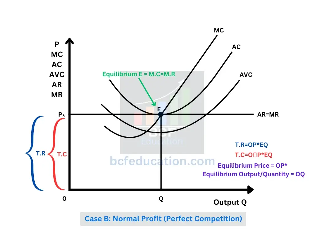
Explanation Case B: Normal Profit
Situation: The firm is making zero economic profit (also known as “breaking even” or earning a “normal profit,” which is the minimum return required to keep the firm in business).
Why? The market price (OP*) is exactly equal to the firm’s Average Cost (AC) at the equilibrium output (OQ).
Graphical Analysis:
The price line (AR=MR) is tangent to the lowest point of the AC curve at point E.
TR = Area OP*EQ
TC = Area OPEQ (since AC = P at that point).
Profit = TR – TC = 0
Conclusion: The firm is covering all its costs, including the opportunity cost of capital, and has no incentive to enter or exit the market. This is a long-run equilibrium point.
Case C: Normal Loss

Explanation Case C: Normal Loss (Subnormal Profit)
Situation: The firm is incurring a loss, but it should continue operating in the short run.
Why? The market price (OP*) is below Average Cost (AC) but above Average Variable Cost (AVC).
Graphical Analysis:
At output OQ, price P* (point E) is less than AC (point B) but greater than AVC.
TR = Area OP*EQ
TC = Area OABQ (since AC at OQ is at point A).
Loss = TC – TR = Area P*EBA
Fixed Cost: The diagram correctly splits this loss. The firm uses part of its revenue to cover some of its fixed costs.
The green area P*ECD represents the portion of fixed costs covered by revenue.
The red area ABPE (which is the same as the total loss PEBA) represents the unrecovered fixed costs, which is the “normal loss.”
Conclusion: By producing, the firm generates enough revenue to cover all its variable costs and some of its fixed costs. If it shuts down, it would lose all its fixed costs. Therefore, it is better to operate at a loss.
Case D: Abnormal Loss

Explanation Case D: Abnormal Loss / Shut-Down Point
Situation: The firm is at the point where it should stop production (shut down).
Why? The market price (OP*) is equal to the Minimum of the Average Variable Cost (AVC) curve.
Graphical Analysis:
The price line (AR=MR) touches the AVC curve at its minimum point (E).
At this price, the firm’s TR (OP*EQ) is exactly equal to its Total Variable Cost (TVC). This means it is covering only its variable costs.
It is losing all of its fixed costs (the gap between AC and AVC). The loss is the entire fixed cost amount, labeled as area ABP*E.
Conclusion: The firm is indifferent between producing and shutting down. In both cases, its loss will be exactly equal to its total fixed costs. If the price drops any lower, the firm will minimize its losses by shutting down completely, as it would not even cover its variable costs.
Core Concepts for All Cases
Equilibrium Condition: In all diagrams, the firm’s equilibrium is where Marginal Cost (MC) = Marginal Revenue (MR). This point (labeled ‘E’) determines the profit-maximizing or loss-minimizing output level (OQ).
Price Taker: The firm is a price taker, so the price is set by the market. This is why the Demand (AR) / MR curve is a horizontal straight line at the market price (OP*).
AR (Average Revenue) = Price
MR (Marginal Revenue) = Price
Therefore, AR = MR
Cost Curves:
MC (Marginal Cost): The U-shaped curve.
AC (Average Cost): The U-shaped curve, always above the AVC.
AVC (Average Variable Cost): The U-shaped curve, lying below the AC.
Profit/Loss Calculation:
Total Revenue (TR) = Price × Quantity = Area of [OP × OQ]*
Total Cost (TC) = Average Cost × Quantity = Area of [Average Cost at quantity OQ × OQ]
Profit = TR – TC
Long Run Equilibrium
Characteristics of Equilibrium under Long Run
1. Equality of Marginal Cost and Marginal Revenue
Equilibrium price and equilibrium output is determined under perfect competition in the long run is same as it is done in the short run. As we know that equilibrium output and price is determined where marginal cost MC curve intersects marginal revenue MR line from below. We can say that:
P = M.C = M.R
2. Normal Profits: Firms earn only normal profits (zero economic profits) because if supernormal profits exist, new firms will enter, increasing supply and driving prices down. Conversely, if losses occur, some firms will exit, reducing supply and raising prices.
3. Equality of Marginal Cost and Average Total Cost:
In the long run, firms operate where marginal cost equals average total cost (ATC), ensuring normal profits: MC=ATC
4. Productive Efficiency: Firms produce at the lowest point of the long-run average cost (LRAC) curve, achieving the most efficient use of resources.

Explanation
At the level of price OP1 and output OQ1, firms are earning abnormal profit in the industry. At this level equilibrium point is E1 where MC intersects the MR1.
Due to abnormal profit, new firms attracts to the industry and they enter, in result price goes down to OP and output OQ and they achieve new equilibrium at point E where MC intersects the MR line. It is the ideal point for the firm for equilibrium where LAC line also tangent to point E.
If firm reduces its price to OP2 at output OQ2, its attain equilibrium at point E2 where MC line cuts MR2 line but here LAC line is above the point so it is not the ideal point for the firm.
Related Posts
Evolving different thoughts of Economics
2.1 Theory of Consumer Behaviour
2.2 Total Utility, Marginal Utility, Point of Satiety & Types of Utilities
2.3 The Law of Diminishing Marginal Utility DMU
2.4 The Law of Equal Marginal Utility EMU
3.1 Demand, Individual Demand, Aggregate Demand, Law of Demand
3.2 Change and Shift in Demand, Extension and Contraction in Demand, Rise and Fall in Demand
3.4 Point and Arc Elasticity of Demand
3.5 Income Elasticity of Demand, Cross Elasticity of Demand
4.2 Extension and Contraction, Rise and Fall in Supply
4.4 What is Equilibrium of Demand and Supply, Market Equilibrium